Stochastic processes and stocks simulation

Please before continue reading, make sure to read the disclaimer at the bottom of this article.

Sometimes names of phenomena do not look like they suit the things they are attached to. In my opinion, that’s the case for stochastic processes.
Stochastic process is a fancy word to describe a collection of random variables, which should represent the path of a certain random variable followed over a period of time.

Stochastic processes are an interesting area of study and can be applied pretty everywhere a random variable is involved and need to be studied. Say for instance that you would like to model how a certain stock should behave given some initial, assumed constant parameters. A good idea in this case is to build a stochastic process.

A personal note: I do not believe these stochastic models actually performs good on stocks… At least not with these basics assumptions which I am going to list. I cannot see the reason why a stock should behave like these processes show. These processes are somehow “deterministic” in the sense that you can reasonably get to know how a stock should behave, financial markets however, have always shown to be irrational, non deterministic, and “explainable” only ex-post. In spite of all this, I still like how this kind of stochastic process works and the graph which comes out at the end looks like a stock! Furthermore I cannot hide that understanding financial markets is intriguing.

The basic assumptions are the following:
-Expected annual return and return volatility are known and constant (This is not realistic, furthermore if volatility is calculated on historical returns, there is no reason to believe it is actually capturing the future behave of the stock)
-Returns are normally distributed (Not realistic either. Returns proved themselves not to be normally distributed and to occur in larger magnitude than forecast)

The model is pretty simple, here it is:

Let’s set our scenario in R and generate the process:

Here is the summary of our 256 generated observation:

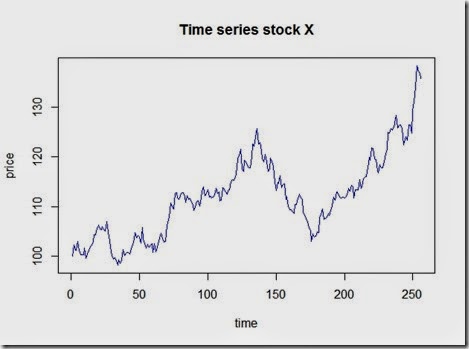
and the plot which looks realistic

Let’s compare this to a pure deterministic model where we assume a constant positive daily return of 30%/255

We can clearly see how the stochastic process uses the deterministic model as a base and then implements random shocks in.

Now, let’s have a look at the distributions

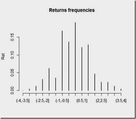
Not that much interesting, not as much as the returns, which we plotted below:

As you can see, returns are approximately normally distributed, and that’s consistent with our assumptions and the methods we used to simulate the changes in prices. It should be wise to note that drastic changes in prices are rare under these assumptions. However, the stock market proved that “extreme events” occur much more frequently than these models suggests. So, are these models to be thrown away? No, the drawings are nice and look similar to the real ones, but aside from this, I believe these models are an interesting starting point worth future development.

---

Disclaimer
This article is for educational purpose only. The numbers are invented. The author is not responsible for any consequence or loss due to inappropriate use. It may contain mistakes and errors. You should never use this article for purposes different from the educational one.