An implementation of the Tic Tac Toe game in Java

Lately I’ve been really busy, and I’ve not had that much time to spend on programming. I’ve had this implementation of the Tic Tac Toe game in my “to do list” for a very long time but sadly for one reason or another it just kept being delayed. In some sense it is easier to code than the text editor I made here, however it has not been so in practice. In particular, I can’t shake the feeling that the code of this project is redundant and sloppy. I’d be happy to be proved wrong but I guess there’s no point in arguing over such a small project.

This project, aside from getting more familiar with Java syntax and its libraries, helped me in becoming more fluent in building a GUI with Swing. There are some technical details which I’d like to discuss perhaps with some professional Java coder in case I get the chance.to talk to one (indeed networking is important).

The main Idea was to develop a Tic Tac Toe implementation and a battleship game as well, however, due to the lack of spare time I put aside the battleship game project and perhaps I will work on it in the future, although the basics of the underlying code are pretty similar to those used here (so similar that it might actually be a repetition).

Enough talk, let’s cut to the chase! Here are some screenshots, and below you can find the download link for the Java application. As usual, I’ve put into the .zip folder the source code so that you can check it out, work on it, whatever you like

How to play:
Basically you click on one of the three columns (if you click on any button on the selected column that’s also fine) and your mark (“x” for the player) is dropped into the lowest box available. Then the computer makes its move (randomly). Whoever reaches first 3 in a row.wins. The idea of the lowest box is due to the fact that I had another game in mind while developing this, it turned out as a “new” kind of Tic Tac Toe and I thought it was nice to play with. Of course by working on the source code I uploaded along with the runnable jar one could easily remove this and get back to the classic game.

Dropbox download link.

Hope this was interesting.

Taylor series with Python and Sympy

Here I am again using my beloved Python and doing maths stuff.

Today I’d like to post a short piece of code I made after a review of Taylor series I did. This script lets you input (almost) any function, provided that it can be represented using Sympy and output the Taylor series of that function up to the nth term centred at x0.

Sympy is a great module for basic symbolic mathematics, it works fine and it is really simple to use even if you are new to Python.

Here is the output of the plot function for the function sin(x) approximating up to the 9th term:

Note that in the console output the series is written backwards, however I think it could be fixed.

Here is the code I used

This code can be customized to return Taylor expansions for any function you’d like to use (of course provided it can be represented using Sympy).

Finally, the code used to generate the plot

My first serious Java project

Finally here I am with my first serious Java project: a text editor!

Yeah I know, perhaps the word “serious” is a bit of an overkill for a simple project such as a text editor. However for a Java newbie, as I consider myself to be, this was actually a middle level project. The hard part was using Swing to implement the user interface, although I find Swing to be easier to use than Tkinter (Python) once that you’ve got the basics.

So, what’s this text editor about? Basically it is a notepad (like the one that comes natively with Windows but with less options, and of course it is written in Java. Here is a screenshot:

Now, let’s talk about how to use this.

The file menu:

The file menu has 4 options: open, show current working directory, set current working directory and exit.
The open command lets you search for a .txt file to display in the user-interface.
The show and change current working directory commands are used to show and change, respectively, the directory you are working in.

You can open a file with the commands “open” and “load .txt file” or work on a new one simply by typing into the white box. When you have edited a file in the text editor, you can save it by typing a name into the bottom text field and then clicking the bottom right button. If you do not enter a name, the file will be saved with a default one. Furthermore, once you click on “save .txt data” the program asks you if you want to save the file in the current working directory. If you need to choose another location click “no” and then choose the directory to save the file in. Enter the same name of the file you are working on, to overwrite it.

The edit menu:

The edit menu basically lets you change font size (by 3 pt a click).

You can download the program (the runnable .jar file and the source code) at this address below:

https://www.dropbox.com/s/e4jhp1w9n1w6pp8/java%20text%20editor.zip?dl=0

Hope this was interesting.

Two simple Java programs

So far I’m still a newbie Java programmer and I am mostly familiar with the basics (the syntax and basic concepts) therefore I thought I could practice my little knowledge by writing two simple programs. In particular, this task helped me to get more familiar with user input, random number generation and arrays. I took the idea from a website, however I lost the bookmark therefore I can not post it.

The first program is quite simple. It asks you to guess a number within 0 and 99. Many improvements could be done to this simple program, perhaps in the future I’ll work on it.

Here it is:

The second program is a little bit more complex, it asks for an input sentence from the user and then it outputs a sentence of the same length using random part of the entered sentence.

Hope this was interesting.

Numerical integration with Python

In this short article I am going to post a simple Python script for numerical integration.

Numerical integration is a part of a family of algorithms for calculating the numerical value of a definite integral. The two simplest method for performing numerical integration are rectangle and trapezoidal rule. If you’d like to know more about these two methods you can check the wikipedia page which has been pretty helpful to me.

Now, the code below works fine if the functions you are using is not decreasing and positive, however:
-If your function is decreasing, the plot need to be adjusted to show the correct graph
-If the function is negative at some point, the code might not work, since it has not been designed to handle it. Perhaps in the future I’ll fix that.

Therefore, bottom line, square root of x is fine, logarithms (after 1),x^2,x^3(from 0) etc…

Here is an approximation with 50 points and the rectangle rule:

and the code output on the console:

Finally, below is the code I used to generate the output above:

Hope this is useful.

Tag di Technorati: maths,python,calculus,algebra,programming,integral,integrals

Volume of solids of revolution: the cone

Have you ever wondered where do all those formulas to calculate the volume of solids like a cone, a cylinder, a sphere ecc… come from? In fact they come from a simple formula and from a clever basic idea. Imagine you have a function f

Intuitively you could approximate the volume by dividing your interval into a number n of small intervals of the same size and sum up the volume of the cylinders of radius f(x) and height , then

if we use an infinite number of steps n then our sum becomes an integral:

Now that we have the intuition, we  can go on to the code. I coded an example in R and one in Matlab. The one in Matlab is shorter since it deals with the integration on its own using symbolic computation while in R I decided to code a simple approximation algorithm based on the first formula I posted above, although you could easily calculate the indefinite integral of the function foo and then use it to calculate the exact volume.

Here is the Matlab example, quick, fast and neat:

Note that f(10)=5, thus the radius of our cone is 5. Furthermore, for the sake of simplicity I’ve assumed that the tip is in 0,0. This code outputs:

Here is the R code. Of course you could have made it shorter and more neat but I like coding in R so I made something more out of it. The R program below approximates the volume using the first approach described above.

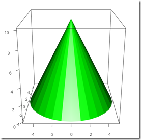
Finally, you can get a 3D cone as the one at the top of this page just by using the RGL package in R and the demo scripts.

Tag di Technorati: geometry,calculus,R,matlab,programming,volume

How to calculate the length of an arbitrary arc

Have you ever wondered if you could calculate how long is a certain curved path with a “simple formula”? Apparently you can, provided that you are good with integrals (or you can use Wolfram Alpha or Matlab). I am no mathematician and this is by no means a rigorous proof, however I think it surely delivers a first grasp on the underlying concepts.

A first approach could be use a real meter, but then you’d have to deal with the uncertainty that comes with every measurement and bla bla bla… From the deep magic forest of calculus, another approach to lines could become very handy: consider for instance an arbitrary curve S

by considering this as a limit in which the change in S approaches ds and applying the Pythagorean theorem we can write:

Now if your line is in parametric form we just divide by dt squared, if it is in the form f(x) then you can divide by dx squared and then integrate with respect to dx. For this example I am assuming S is in parametric form as such:

Dividing by dt squared yields

and after some manipulations we can integrate and get the length of our line from a to b

Suppose we’d like to calculate the length of the arc of our parametric function from 0 to 10, then assuming my calculations are correct, we’d have to calculate

Now perhaps this is easy to calculate manually, perhaps it isn’t, however it is surely fun to implement in some programming language. Sadly the sympy module in Python for symbolic maths does not work on this integral, it just seems to loop forever, perhaps that’s just my computer or I wrote something wrong. Therefore I used Matlab, which, aside from being somewhat difficult to start on my computer, works perfectly for this kind of tasks. In red is the arc whose length we’d like to calculate.

My simple Matlab script spits out as a solution the number 10.7602 which double checked on Wolfram Alpha seems to be the right solution.

To be fair my code prints out this: log(4*410^(1/2) + 81)/8 + 1640^(1/2)/4 which then computed yields the final result. Here below you can check my code

 

Tag di Technorati: maths,matlab,line,integral,programming