(Naive) RSA encryption with Python

Please before continue reading, make sure to read the disclaimer at the bottom of this article.

RSA is a well-known cryptosystem used in many cases where secure data transmission is needed. It basically rely on the also well-known issue of factoring big numbers. As you may recall from high school, each number has a unique prime number factorization. This is the very strength of RSA. In order to decrypt a message encrypted with RSA you would need to factorize a REALLY BIG number and this problem may take a very long time to be solved, it may take so long that it becomes unpractical to be achieved.

If you want to get more on RSA click here.
Here is the algorithm carefully described.

I have always been fascinated by encryption and cryptosystems. For those who did not know, Alan Turing, during the Second World War, devised a machine which made it possible to decrypt Enigma code in relatively short time and therefore gain a significant advantage. This machine was basically the first computer. You can watch this incredible piece of history on you tube. Here are some interesting videos:

Numberphile Enigma video
An interesting documentary

Now let’s get to the necessary premises and the code!
First of all, to start off you need two big primes, p and q. I do not know how they usually get these primes (I haven’t covered it yet) but anyway, they are almost all you need to start your “naive” RSA encrypting system in Python. We will use small numbers for the sake of simplicity and this is basically one of the factors that led me to use the word “naive” since it could be easily broken in a short time.

	import gmpy2
	# Note: you do not need gmpy2 if you use small numbers, you
	# could have also use the built-in pow() function. Check
	# the official documentation for more information on pow()
	number_to_encrypt = 512
	##############################################################
	# SETUP
	# We choose two big primes, here we use small primes
	# for the sake of simplicity
	p = 67
	q = 83
	e = 59
	# Small note: if the number to encrypt has more digits than
	# the modulus the algorithm won't work
	# We find n
	n = p*q
	# and phi(n) which should be coprime with phi(n)
	phi_n = (p-1)*(q-1)
	e = 59
	# This function returns True if coprime_to_check is coprime with phi_n
	def is_coprime_phi(phi_n, coprime_to_check):
	while phi_n % coprime_to_check == 0:
	coprime_to_check = input("Enter a prime number, to check if coprime with phi_n")
	e = coprime_to_check
	return True
	# If e is not coprime with phi(n) ValueError is raised
	if not is_coprime_phi(phi_n,e):
	raise ValueError("e is not coprime with phi_n")
	# The following code finds the modular multiplicative inverse
	def egcd(a, b):
	if a == 0:
	return (b, 0, 1)
	else:
	g, y, x = egcd(b % a, a)
	return (g, x - (b // a) * y, y)
	def modinv(coprime, phi_n):
	g, x, y = egcd(coprime, phi_n)
	if g != 1:
	raise Exception('modular inverse does not exist')
	else:
	return x % phi_n
	# The modular multiplicative inverse
	d = modinv(e,phi_n)
	# Public key
	pub_k = [e,n]
	# Private key
	priv_k = [d,n]
	# Encrypting and decrypting functions
	def encrypt_this(m):
	result = gmpy2.powmod(m,e,n)
	return result
	def decrypt_this(c):
	plain = gmpy2.powmod(c,d,n)
	return plain
	###########################################################
	# Encrypt
	enc = encrypt_this(number_to_encrypt)
	print("Encypted number: ",enc)
	# Decrypt
	dec = decrypt_this(enc)
	print("Decrypted plain number: ",dec)

view raw naive_rsa.py hosted with ❤ by GitHub

Here is the result which should be printed out:

Therefore, hypothetically, Bob, who needs to send a message (512) to Alice, would use Alice’s public key to encrypt 512 and then send her the number 477. Alice would then use her private key to decrypt 477 and get back 512, the original message.

Hope this was interesting.

---

Disclaimer: This article is for educational purpose ONLY. If you need a security system you should ask to professionals who are competent in the field. The author of the article is by no means a professional or an expert in this field and might, therefore, make big mistakes. This code must NOT be used for anything other than educational purpose. The provider of this code does not guarantee the accuracy of the results and accepts no liability for any loss or damage that may occur as a result of the use of this code. Understanding and agreeing to the terms of this disclaimer is a condition of use of this code. By reading the article you confirm you have understood and will comply with this disclaimer.

Plain vanilla BlackJack simulation with R

Please before continue reading, make sure to read the disclaimer at the bottom of this article.

Here is a simulation I run with R in the same period I created the poker one.

I have just decided to call it plain vanilla since neither double down or split pairs are allowed. Rules are as basic as they can be.

The code looks like messy, I know, If I had to do it now, I guess I would do many things differently, however, the results looks fine, and the code runs fine as well, therefore it is not entirely to be thrown away I believe.

The simulation is divided in two parts. In the first one I looked for the probabilities for each possible event (that’s to say: “player wins”, “tie”, “dealer wins”). Since the code looks pretty hairy, many explanations are provided.

A small but important note: if you want to run the simulation, since it is a bit demanding computationally speaking, in order not to crash RStudio you may want to run a line a time and not the entire code all at once, or just maybe use only some functions, just be careful because since we run the simulation a big number of times and the functions are not the fastest to be run, your computer might complain a little.

Here is the code:

	# In this example we simulate a plain vanilla Blackjack game
	# and we calculate the probabilites of win and tie for both the player and the dealer
	# A deck of 52 cards (Jokers are excluded), A is an ace.
	# Please note: as in BlackJack figures worth 10 each, we will deal with each picture as if it were a ten
	deck = c("A","A","A","A",10,10,10,10,10,10,10,10,10,10,10,10,10,10,10,10,9,9,9,9,8,8,8,8,7,7,7,7,6,6,6,6,5,5,5,5,4,4,4,4,3,3,3,3,2,2,2,2)
	# Usually, in casinos, Blackjack games are played
	# with 4 to 6 decks. The following function will take in
	# account this matter and return the appropriate deck
	# according to the number the casino uses (n)
	deck_in_use <- function(n)
	{
	deck_to_return = rep(deck,n)
	return(deck_to_return)
	}
	# The function hand takes a deck and returns a hand of Blackjack
	hand <- function(deck_to_use, player_hand)
	{
	# We fix player's hand
	p_hand = player_hand
	# We fix the deck
	deck = deck_to_use
	# Player's hand gets removed from the deck,
	# since it is no longer available to be dealt
	for(i in p_hand)
	{
	if(is.element(i,deck))
	{
	deck<-deck[-match(i,deck)]
	}
	}
	# In case player's hand contains aces, the following
	# code trasforms aces in 11 or 1 according to BJ rules
	if((p_hand[1]) == "A" &amp;&amp; (p_hand[2] == "A"))
	{
	p_hand[1] <- 1
	p_hand[2] <- 11
	}else if((p_hand[1] == "A") && (p_hand[2] != "A"))
	{
	p_hand[1] <- 11
	}else if((p_hand[2] == "A") &amp;&amp; (p_hand[1] != "A"))
	{
	p_hand[2] <- 11
	}
	p_hand <- as.numeric(p_hand)
	# Dealer's drawing function: if dealer's hand is
	# lower than 16, then another card is dealt
	d_draw <- function(hand)
	{
	if(sum(hand) > 16)
	{
	return(hand)
	}else
	{
	new_card = sample(deck,1,F)
	hand = append(hand,new_card)
	if(is.element(new_card, deck))
	{
	deck<-deck[-match(new_card, deck)]
	}
	# In case the newly dealt card is an ace,
	# the following code deals with it
	if(new_card == "A")
	{
	place_holder_ace_d2 <- match(new_card, hand)
	vect_partial_sum_hand = hand[-place_holder_ace_d2]
	vect_partial_sum_hand <- as.numeric(vect_partial_sum_hand)
	if(sum(vect_partial_sum_hand) <= 10)
	{
	hand[place_holder_ace_d2] <- 11
	}else
	{
	hand[place_holder_ace_d2] <- 1
	}
	}
	hand <- as.numeric(hand)
	# In case something went missing from before,
	# the following code checks if every ace has
	# the appropriate value
	hand_minus_new_card &lt;- hand[-match(new_card, deck)]
	if((sum(hand) <= 21) && (is.element(11,hand_minus_new_card)))
	{
	hand[match(11, hand)] <- 1
	}
	hand <- as.numeric(hand)
	# Redraw is needed in case dealer's hand is lower than 16
	return(d_draw(hand))
	}
	}
	# Dealer's hand is eventually sampled and implemented with the
	# d_draw function to simulate a real draw.
	dealer_hand <- function()
	{
	hand = sample(deck,2,F)
	for(i in hand)
	{
	if(is.element(i,deck))
	{
	deck<-deck[-match(i,deck)]
	}
	}
	# If the dealer has two Aces they are converted into a 11 and a 1
	if((hand[1] == "A") && (hand[2] == "A"))
	{
	hand[1] <- 11
	hand[2] <- 1
	hand <- as.numeric(hand)
	}else
	{
	# If an A is in the dealer hand, it is converted into an 11
	for(i in hand)
	{
	place_holder_ace_d <- match(i, hand)
	if(i == "A")
	{
	hand[place_holder_ace_d] <- 11
	}
	}
	hand <- as.numeric(hand)
	}
	hand <- d_draw(hand)
	return(hand)
	}
	# Results are eventually collected into a list and returned by the function
	results = list(p_hand, dealer_hand())
	return(results)
	}
	# The following function simulates n Blackjack hands and store the
	# results in a matrix. It returns some probabilities (please check below)
	# n is the number of hands to be played in the simulation
	simulate_games<;- function(deck_to_use, player_hand, n)
	{
	names_ <- c("Dealer","Player", "Test_win", "Test_draw")
	result_matrix <- matrix(ncol = 4)
	colnames(result_matrix) <- names_
	for(i in 1:n)
	{
	game <- hand(deck_to_use,player_hand)
	vec_result <- c(sum(game[[2]]), sum(game[[1]]))
	draw <- (vec_result[2] == vec_result[1])
	# Tie
	if(draw)
	{
	vec_result[3] <- 0
	vec_result[4] <- 1
	result_matrix <- rbind(result_matrix, vec_result)
	# Dealer hits Blackjack
	}else if((vec_result[1] == 21) && (length(game[[1]]) == 2) &&; (vec_result[2] != 21) )
	{
	vec_result[3] <- 0
	vec_result[4] <- 0
	result_matrix <- rbind(result_matrix, vec_result)
	# Player wins on points
	}else if((vec_result[2] < vec_result[1]) | (vec_result[1] < 21))
	{
	vec_result[3] <- 1
	vec_result[4] <- 0
	result_matrix <- rbind(result_matrix, vec_result)
	# Dealer wins
	}else
	{
	vec_result[3] <- 0
	vec_result[4] <- 0
	result_matrix <- rbind(result_matrix, vec_result)
	}
	}
	# Delete first row of the results matrix
	result_matrix <- result_matrix[-1,]
	# Show results matrix
	#View(result_matrix)
	probab_win = sum(result_matrix[,3])/n
	probab_tie = sum(result_matrix[,4])/n
	probab_dealer_win = 1 - probab_win - probab_tie
	#name_data <- c("Prob of win", "Prob of a tie", "Prob of dealer win")
	vect_data <- c(probab_win, probab_tie, probab_dealer_win)
	#names(vect_data) <- name_data
	return(vect_data)
	}
	# Simulation with 3 decks a hand equal to 19 and 100 games
	# Sidenote: this game is as if the dealer was shuffling the
	# cards at each game
	simulate_games(deck_in_use(3), c(10,9), 100)
	# Simulation of n_games*n_hand_game with n_deck decks and a hand equal to hand
	simulate_n_games &lt;- function(n_deck, hand, n_hand_game, n_games)
	{
	res_matrix <- matrix(ncol = 3)
	names = c("prob of win", "prob of tie", "prob of dealer win")
	colnames(res_matrix) &lt;- names
	for(i in 1:n_games)
	{
	data_vec <- simulate_games(deck_in_use(n_deck), hand, n_hand_game)
	res_matrix <- rbind(res_matrix, data_vec)
	}
	res_matrix <- res_matrix[-1,]
	View(res_matrix)
	probab_win <- sum(res_matrix[,1])/nrow(res_matrix)
	probab_tie <- sum(res_matrix[,2])/nrow(res_matrix)
	probab_dealer_win &lt;- 1 - probab_win - probab_tie
	probabilities <- c(probab_win, probab_tie, probab_dealer_win)
	name_data <- c("Prob of win", "Prob of a tie", "Prob of dealer win")
	names(probabilities) <- name_data
	return(probabilities)
	}
	# Simulate 2000*100 Blackjack games with 3 decks and a hand equal to 18
	simulate_n_games(3,c(10,8),2000,100)
	# You may want to run the following lines one a time since they
	#are a little "heavy" to compute.
	# The simulation is run for hands from 16 to 21
	first_row_16 <- simulate_n_games(3,c(10,6),2000,100)
	second_row_17 <- simulate_n_games(3,c(10,7),2000,100)
	third_row_18 <- simulate_n_games(3,c(10,8),2000,100)
	fourth_row_19 <- simulate_n_games(3,c(10,9),2000,100)
	fifth_row_20 <- simulate_n_games(3,c(10,10),2000,100)
	sixth_row_21 <- simulate_n_games(3,c(10,11),2000,100)
	BJ_probabilities <- matrix(ncol = 3)
	BJ_probabilities <- rbind(BJ_probabilities,first_row_16)
	BJ_probabilities <- rbind(BJ_probabilities,second_row_17)
	BJ_probabilities <- rbind(BJ_probabilities,third_row_18)
	BJ_probabilities <- rbind(BJ_probabilities,fourth_row_19)
	BJ_probabilities <- rbind(BJ_probabilities,fifth_row_20)
	BJ_probabilities <- rbind(BJ_probabilities,sixth_row_21)
	BJ_probabilities <- BJ_probabilities[-1,]
	View(BJ_probabilities)
	hands_points <- c(16,17,18,19,20,21)
	plot(hands_points, BJ_probabilities[,1], xlab = "Hands full points", main = "Probability of player win", type = "b", col="blue")
	plot(hands_points, BJ_probabilities[,2], xlab = "Hands full points", main = "Probability of tie", type = "b", col="blue")
	plot(hands_points, BJ_probabilities[,3], xlab = "Hands full points", main = "Probability of dealer win", type = "b", col="blue")

view raw blackJack_simulation1.R hosted with ❤ by GitHub

Let’s have a look at the results that we have got:

By simply standing with a hand equal to 19, you can expect to win 59% of the times, and loose 28%. A tie is likely to occur 13% of the times.

Let’s now simulate 2000*100 games with a hand equal to 18 and 3 decks and then average the probabilities:

In this case the odds seem to be a lot worse than before, by just subtracting 1 point to the player’s hand we raised the probability of win for the dealer from 28% to 43.4%.

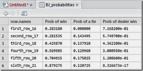
Why not run the simulation for each hand from 16 to 21 and then plot the results? Warning: your computer may yell at you after this demanding step!

As we could expect, as the player’s hand gets higher, the probabilities of winning increases. For some reason which I ignore, R did not print in plain the probabilities of winning for the dealer, however you can easily get them from the table above or by calculating for each row 1 - Prob of Win – Prob of a tie, since the three events should (must) sum up to one. It is interesting to note that the probability of a tie is more or less near 12-14% and that, as we expected, it is equal to 0 when the hand is equal to 16 (since the dealer must draw on 16 and therefore a tie is not possible).

Here are the plots:

This is the end of part 1 of the simulation.

 

---

And now the second part. Here we want to know what are the probabilities of not bust when we draw 1 or 2 cards given a certain hand.

	# In this example we calculate the probabilities of bust
	# and survival by asking for 1 or 2 cards given a hand
	# Auxiliary functions are set first
	# This function gives a player hand after n_draw given a hand,
	# n decks, and a fixed number of draw (hits). Note: hand is a vector
	hand_to_try <- function(n_decks, hand, n_draw)
	{
	deck_to_use <- deck_in_use(n_decks)
	# Player's hand gets removed from the deck, since it is no longer available
	for(i in hand)
	{
	# Remove aces
	if((i == 11) | (i == 1))
	{
	deck_to_use <- deck_to_use[-match("A", deck_to_use)]
	}else
	{
	deck_to_use <- deck_to_use[-match(i, deck_to_use)]
	}
	}
	# Dealer draws
	dealer_hand <- hand(deck_to_use, hand)[[2]]
	# Dealer's hand gets removed from the deck, since it is no longer available
	for(i in dealer_hand)
	{
	# remove aces
	if((i == 11) | (i == 1))
	{
	deck_to_use <- deck_to_use[-match("A", deck_to_use)]
	}else
	{
	deck_to_use <- deck_to_use[-match(i, deck_to_use)]
	}
	}
	# Assuming hand is <= 11, n_draw cards are dealt and added to player's hand
	for(i in 1:n_draw)
	{
	new_card <- sample(deck, 1, F)
	if(new_card == "A")
	{
	new_card <- 1
	new_card <- as.numeric(new_card)
	}
	hand <- append(hand, new_card)
	}
	# the function returns the final hand for the player
	return(hand)
	}
	# Here we try the function
	hand_to_try(1,c(10,"A"),2)
	# This function simulates n_games trial at drawing n_draw
	# cards given a player's hand with n_decks BJ game
	# and returns the matrix with all the hands
	m_pbusted_afterndraw <- function(n_games, n_decks, hand, n_draw)
	{
	hand_matrix <- matrix(ncol = length(hand) + n_draw)
	for(i in 1:n_games)
	{
	p_hand <- hand_to_try(n_decks, hand, n_draw)
	hand_matrix <- rbind(hand_matrix, p_hand)
	}
	#View(hand_matrix)
	hand_matrix <- hand_matrix[-1,]
	#View(hand_matrix)
	return(hand_matrix)
	}
	# This code generates a matrix of 200 hands with two draws
	# with a hand of 15 and 2 decks
	matrix_hands <- m_pbusted_afterndraw(200, 2, c(10,5),2)
	# This function, given a matrix of hands as matrice_hands,
	# simply calculates the frequency (probability) of bust and not bust.
	probab_bust <- function(matrix)
	{
	result_matrix <- matrix(ncol = 2)
	colnames(result_matrix) <- c("Busted", "Not busted")
	#In the matrix, 1 = True, 0 = False
	for(i in 1:nrow(matrix))
	{
	if(sum(as.numeric(matrix[i,])) < 21)
	{
	result_matrix <- rbind(result_matrix, c(1,0))
	}else
	{
	result_matrix <- rbind(result_matrix, c(0,1))
	}
	}
	result_matrix <- result_matrix[-1,]
	#View(result_matrix)
	probab_vect <- c(sum(result_matrix[,1])/nrow(result_matrix), sum(result_matrix[,2])/nrow(result_matrix))
	names(probab_vect) <- c("Probability of Bust", "Probability of survival")
	return(probab_vect)
	}
	probab_bust(matrix_hands)
	# The following code simulates 1000 hands each, with 3 decks,
	# a hand (from 10 to 17) and one hit (draw), they return a matrix each
	matrice_hands_hand_11_1draw <- m_pbusted_afterndraw(1000, 3, c(9,2),1)
	matrice_hands_hand_12_1draw <- m_pbusted_afterndraw(1000, 3, c(9,3),1)
	matrice_hands_hand_13_1draw <- m_pbusted_afterndraw(1000, 3, c(9,4),1)
	matrice_hands_hand_14_1draw <- m_pbusted_afterndraw(1000, 3, c(9,5),1)
	matrice_hands_hand_15_1draw <- m_pbusted_afterndraw(1000, 3, c(9,6),1)
	matrice_hands_hand_16_1draw <- m_pbusted_afterndraw(1000, 3, c(9,7),1)
	matrice_hands_hand_17_1draw <- m_pbusted_afterndraw(1000, 3, c(9,8),1)
	# The following code simulates 1000 hands each, with 3 decks,
	# a hand (from 10 to 17) and two hits (2 new cards), they return a
	# matrix each
	matrice_hands_hand_10_2draw <- m_pbusted_afterndraw(1000, 3, c(9,1),2)
	matrice_hands_hand_11_2draw <- m_pbusted_afterndraw(1000, 3, c(9,2),2)
	matrice_hands_hand_12_2draw <- m_pbusted_afterndraw(1000, 3, c(9,3),2)
	matrice_hands_hand_13_2draw <- m_pbusted_afterndraw(1000, 3, c(9,4),2)
	matrice_hands_hand_14_2draw <- m_pbusted_afterndraw(1000, 3, c(9,5),2)
	matrice_hands_hand_15_2draw <- m_pbusted_afterndraw(1000, 3, c(9,6),2)
	matrice_hands_hand_16_2draw <- m_pbusted_afterndraw(1000, 3, c(9,7),2)
	matrice_hands_hand_17_2draw <- m_pbusted_afterndraw(1000, 3, c(9,8),2)
	# The following code calculates the probabilities of bust for
	# the two sets of arrays
	prob_bust_hand_11_1draw <- probab_bust(matrice_hands_hand_11_1draw)
	prob_bust_hand_12_1draw <- probab_bust(matrice_hands_hand_12_1draw)
	prob_bust_hand_13_1draw <- probab_bust(matrice_hands_hand_13_1draw)
	prob_bust_hand_14_1draw <- probab_bust(matrice_hands_hand_14_1draw)
	prob_bust_hand_15_1draw <- probab_bust(matrice_hands_hand_15_1draw)
	prob_bust_hand_16_1draw <- probab_bust(matrice_hands_hand_16_1draw)
	prob_bust_hand_17_1draw <- probab_bust(matrice_hands_hand_17_1draw)
	prob_bust_hand_10_2draw <- probab_bust(matrice_hands_hand_10_2draw)
	prob_bust_hand_11_2draw <- probab_bust(matrice_hands_hand_11_2draw)
	prob_bust_hand_12_2draw <- probab_bust(matrice_hands_hand_12_2draw)
	prob_bust_hand_13_2draw <- probab_bust(matrice_hands_hand_13_2draw)
	prob_bust_hand_14_2draw <- probab_bust(matrice_hands_hand_14_2draw)
	prob_bust_hand_15_2draw <- probab_bust(matrice_hands_hand_15_2draw)
	prob_bust_hand_16_2draw <- probab_bust(matrice_hands_hand_16_2draw)
	prob_bust_hand_17_2draw <- probab_bust(matrice_hands_hand_17_2draw)
	# The final array for 1 draw is built
	bust_p_array_1draw <- matrix(ncol = 2)
	bust_p_array_1draw <- rbind(bust_p_array_1draw, prob_bust_hand_11_1draw)
	bust_p_array_1draw <- rbind(bust_p_array_1draw, prob_bust_hand_12_1draw)
	bust_p_array_1draw <- rbind(bust_p_array_1draw, prob_bust_hand_13_1draw)
	bust_p_array_1draw <- rbind(bust_p_array_1draw, prob_bust_hand_14_1draw)
	bust_p_array_1draw <- rbind(bust_p_array_1draw, prob_bust_hand_15_1draw)
	bust_p_array_1draw <- rbind(bust_p_array_1draw, prob_bust_hand_16_1draw)
	bust_p_array_1draw <- rbind(bust_p_array_1draw, prob_bust_hand_17_1draw)
	bust_p_array_1draw <- bust_p_array_1draw[-1,]
	View(bust_p_array_1draw)
	# The final array for 2 draw is built
	bust_p_array_2draw <- matrix(ncol = 2)
	bust_p_array_2draw <- rbind(bust_p_array_2draw, prob_bust_hand_11_2draw)
	bust_p_array_2draw <- rbind(bust_p_array_2draw, prob_bust_hand_12_2draw)
	bust_p_array_2draw <- rbind(bust_p_array_2draw, prob_bust_hand_13_2draw)
	bust_p_array_2draw <- rbind(bust_p_array_2draw, prob_bust_hand_14_2draw)
	bust_p_array_2draw <- rbind(bust_p_array_2draw, prob_bust_hand_15_2draw)
	bust_p_array_2draw <- rbind(bust_p_array_2draw, prob_bust_hand_16_2draw)
	bust_p_array_2draw <- rbind(bust_p_array_2draw, prob_bust_hand_17_2draw)
	bust_p_array_2draw <;- bust_p_array_2draw[-1,]
	View(bust_p_array_2draw)
	hands_points <- c(11,12,13,14,15,16,17)
	plot(hands_points, bust_p_array_1draw[,1], xlab = "Starting hand", main = "Probability of bust \ndrawing 1 card given \na BJ hand", type = "b", col="red")
	plot(hands_points, bust_p_array_1draw[,2], xlab = "Starting hand", main = "Probability of survival \ndrawing 1 card given \na BJ hand", type = "b", col="blue")
	plot(hands_points, bust_p_array_2draw[,1], xlab = "Starting hand", main = "Probability of bust \ndrawing 2 cards given \na BJ hand", type = "b", col="red")
	plot(hands_points, bust_p_array_2draw[,2], xlab = "Starting hand", main = "Probability of survival \ndrawing 2 cards given \na BJ hand", type = "b", col="blue")

view raw blackJack_simulation2.R hosted with ❤ by GitHub

Let’s have a look at the new results we have got:
This is a hand we have got by asking 2 times card from a single deck.

with a starting hand equal to (10,”A”) if we were to ask 2 cards, here are the probabilities that we should face:

Eventually, we can compute the probabilities of “survival” and bust for each hand from 16 to 17 and plot the results.

The results looks pretty interesting and it is nice to see that the probability of bust if we ask for 1 card and our starting hand is 11 is 0 as we could easily predict, however, if we were to ask 2 cards, our chances of survival would suddenly drop to 25%. A big leap!

Hope this was interesting.

---

Disclaimer: This article is for educational purpose ONLY. Odds generated by this code are calculated by a random simulation. As such the odds will represent an approximation of the true odds. They might even be completely wrong or misleading. This code must NOT be used for anything other than educational purpose. The provider of this code does not guarantee the accuracy of the results and accepts no liability for any loss or damage that may occur as a result of the use of this code. Understanding and agreeing to the terms of this disclaimer is a condition of use of this code. By reading the article you confirm you have understood and will comply with this disclaimer.

A BlackJack game simulator with Python

Hi everyone! Here is another one of the first projects I have developed. The project is quite simple as the name tells: A blackJack game simulator.

The modules used to build this game are the following:
-The Random module, mainly the sample function to sample from a deck of 52 cards.
-EasyGui. Again, another one such as tkinter would have probably been better however I did not know even the name of tkinter at the time I built this.

Some notes on the game:
-Double down is allowed
-The scores are the same as most real BlackJack games
-You can set your initial amount available and the maximum bet (you could even set a negative bet I guess it should work even in that case ah ah).
-There still no insurance available and splitting is not allowed (perhaps I will implement this when I’ll improve the GUI)

IMPORTANT NOTE: Please, before running the script with Python make sure to set the path to the folder where the images are located so that they can appear on the EasyGui window.

You can download the source code here.

Here are some screenshots

Hope you enjoy.

Letter frequency with Python

Let’s say that your favourite subject is languages and comparisons between different languages, or that you enjoy as a hobby decrypting simple codes. Well then, with Python you have found the right tool to use!

Letter frequency, however, is a topic studied in cryptanalysis and has been studied in information theory to save up the size of information to be sent and prevent the loss of data. In fact if the most frequent letter in a language is, say “e”, then it is convenient to use the “least expensive” (in terms of amount of information) way to send that piece of information by reducing the number of bytes sent. For instance, if you were to send binary code, you could use the number 0 to represent “e”.
This is a basic underlying idea in many famous codes. If you would like to get a short introduction to this topic, check this video.

Another example, which uses techniques based on a similar concept is data-compression. Check this great video for a general introduction to data-compression.

Some encryption techniques, such as Caesar cipher and other basic ciphers, can be easily decrypted by spotting the frequency of occurrence of each character and then “guessing” what it should represent by comparing its frequency to the frequency of letters in the language the original message was written in. In fact, this decryption technique can be used for each encryption method which does not uses different symbols to represent the different occurrence of the same character. What do I mean by this? Well, imagine that you need to encrypt this: “bbbb”, now, if you decide to use a Caesar cipher and say, using a shift of 23, your encrypted message will look something like this “yyyy”. Each additional “b” will be converted into a “y” no matter what. This is a soft spot of all those encryption techniques which follows similar schemes.

By using Python, you can easily build a program to run through a long string of text and then calculate the relative frequency of occurrence of each character. Below is the code I used to build this simple program:

	# The following code takes as input a string of text, and then it outputs the barplot of the
	# frequencies of occurrence of letters in the string.
	import pylab as pl
	import numpy as np
	string1 = """ Example string """
	alphabet = ["a","b","c","d","e","f","g","h","i","j","k","l","m","n","o","p","q","r","s","t","u","v","w","x","y","z",".",",",";","-","_","+"]
	# The following functon takes a list and a string of characters, it calculates how often a certain character appears
	# and then it outputs a list with character and frequency
	def frequencies(string,letters):
	list_frequencies = []
	for letter in letters:
	freq = 0
	for i in string:
	if i == letter:
	freq += 1
	if freq != 0:
	list_frequencies.append(letter)
	list_frequencies.append(freq)
	return list_frequencies
	print(frequencies(string1,alphabet))
	# This function returns a list containing 2 lists with letter and frequencies
	def fix_lists_letter(list_1):
	list_letters = []
	list_letters.append(list_1[0])
	list_freq = []
	for i in range(1,len(list_1)):
	if i % 2 == 0:
	list_letters.append(list_1[i])
	else:
	list_freq.append(list_1[i])
	if len(list_letters) != len(list_freq):
	return "Some error occurred"
	else:
	final_list = [list_letters,list_freq]
	return final_list
	first_count = frequencies(string1,alphabet)
	final = fix_lists_letter(first_count)
	letter_s = final[0]
	freq = final [1]
	print("Number of character used:",sum(freq), sep=" ")
	# Enable the following to sort (in descending order)
	"""
	#The follwing function sorts the letters and frequencies in descending order.
	def sort_all(c):
	letters = c[0]
	freq = c[1]
	final_letter = []
	final_freq = []
	for i in range(0,len(letters)):
	maximum = max(freq)
	ind = freq.index(maximum)
	final_freq.append(freq[ind])
	final_letter.append(letters[ind])
	letters.remove(letters[ind])
	freq.remove(freq[ind])
	to_return = [final_letter,final_freq]
	return to_return
	the_very_final = sort_all(final)
	letter_s = the_very_final[0]
	freq = the_very_final[1]"""
	# Relative frequencies
	def get_rel_freq(list_1):
	list_to_ret = []
	for i in list_1:
	list_to_ret.append(i/sum(list_1))
	return list_to_ret
	freq = get_rel_freq(freq)
	fig = pl.figure()
	ax = pl.subplot(111)
	width=0.8
	ax.bar(range(len(letter_s)), freq, width=width)
	ax.set_xticks(np.arange(len(letter_s)) + width/2)
	ax.set_xticklabels(letter_s, rotation=45)
	pl.show()

view raw letter_frequency.py hosted with ❤ by GitHub

Once I built the code, I ran it a couple of times on some wikipedia pages written in English, French, Italian and German, below you can find the results of this process. I should mention that my code missed a lot of characters like è,é,à,ò,ù and the german umlaut. However you can easily add these by simply adding them to the alphabet list. On the y axes is represented the relative frequency of occurrence (in percentage).

And the same graphs sorted.

I do not know if there is a given distribution for each language, I doubt this, however we can clearly see that some letters are much more frequent than others. The letter “e” seems to be pretty common in all the four languages.

Hope this was interesting.

Calculating VaR with R

Simulations can be useful in an unimaginably large number of scenarios. Finance in particular is a field of study where maths and statistics have made led to great advances (sometimes for the good, sometimes for the bad). Value at Risk is just another example of subject where a simulation approach could be handy.

But, what is VaR? VaR is an indicator used in risk management, it represents the maximum potential loss which can occur to a portfolio of a certain investor, say 95% of the times. Well, actually, it could be better to say that 5% of the times the loss will be larger than what VaR predicted (and it could be way larger). In this case we say that we are calculating VaR with 5% confidence.

There are at least three ways of calculating VaR:
-Parametric VaR
-Historical VaR
-Monte Carlo VaR

Let’s see each of them. For simplicity we will assume that our hypothetical investor has only one type of stock in their portfolio and that the holding period N is equal to 1.

Parametric VaR: Here is the formula

Where W0 is the value of the portfolio at time of calculation, N is the holding period, sigma is the daily volatility and Z is the inverse of the normal distribution for 1 minus alpha which is the confidence level. (If alpha is 5% then Z is approximately –1.64, note however that VaR is a positive quantity). The use of the normal distribution of course hides important assumptions which often are fundamental for the reliability of these methods.

Historical VaR:

HR are the historical returns and Percentile is the quantile function in R applied to the historical returns. Note that there is no square root of N, since the holding period is equal to 1. If holding period > 1 day you should multiply this for N as above.

Monte Carlo VaR:
With this approach you simulate a stochastic process which represent the path of the stock and then once you have calculated the logarithmic returns you just check the 5% percentile return and multiply it for the value of the portfolio at time 0.

Let’s see how to implement all this in R. The data used has been invented, and is downloadable from here

	c <- read.csv("C:/users/username/desktop/table.csv",header=T)
	attach(c)
	# View data
	Open
	n <-length(Open)
	i = 1
	rend <- c(0)
	# Calculating logarithmic returns
	while(i < n)
	{
	r <- log(Open[i]/Open[i+1],exp(1))
	rend[i] <- r
	i = i + 1
	}
	# A summary of the returns (in percentage)
	summary(rend*100)
	# View returns table
	View(rend)
	data <- c(length(Open),mean(Open),mean(rend),sd(rend),255*mean(rend))
	names(data) <- c("Total days","Average price","Daily change","Daily volatility","Annualized rr 255gg")
	data
	# Daily volatility
	vol <- data[4]
	# Daily average return
	rendd <- data[3]
	# VaR calculation
	az <- 1000 # Number of stocks
	value1 <- Open[1] # Actual price
	valuep <- value1*az # Value of portfolio
	hp <- 1 # Holding period
	a <- .95 # Confidence level (5%)
	# Parametric VaR
	parvar <- abs(valuep*qnorm(1-a,0,1)*vol*sqrt(hp))
	# Historical VaR
	hvar <- abs(quantile(rend,1-a)*valuep)
	# Vector comparing the two VarS
	varv <- c(parvar,hvar)
	names(varv)<- c("parametric VaR","Historical VaR")
	print(varv)
	detach(c)

view raw var_R.R hosted with ❤ by GitHub

Here are some results:

The results tells us that our investor should experience losses greater than 2835.56 (or 1843.85) only 5% of the times. Usually this two values should not differ that much, however, considering how they are structured and that the data I used is completely made up and too short for historical VaR, it is still fine that we got these results. Usually the time series from which data is gathered are very long, the longer the series the more precise the result. In the last version of VaR, once simulated the behaviour of the stock you just calculate the logarithmic returns and then take out the 95% percentile.

For more information, check the wikipedia page here.

---

Disclaimer
This article is for educational purpose only. The numbers are invented. The author is not responsible for any consequence or loss due to inappropriate use. It can contain mistakes and errors. You should never use this article for purposes different from the educational one.

A simple roulette game simulator created with Python

Another project! This is one of the first game simulator I have tried to develop with Python. It’s basically a roulette simulator and has all the features a roulette should has, I guess!

Some notes:
-The roulette has only one zero (no double zero)
-Payoff are the same as a real roulette (no real money is involved, of course!)
-Outcomes should be uniformly distributed
-The graphics is not the best due to the fact that I used Easygui. Perhaps in the future I will implement the game with tkinter.

Here are the modules used:
-Random. The random module is necessary to simulate the random spin of the roulette.
-Easygui for the graphics. Easygui is a very simple module for user-interaction. I believe it is built on tkinter but has way less features. If you are new to GUI programming in Python I suggest starting with either tkinter or wxPython but not Easygui. Easygui is easier but not that useful nor customizable. On the contrary, the other two modules are harder to use for a new programmer but way more customizable and “complete”. Also the playability is somewhat ruined by the appearing and disappearing windows by Easygui.

You can download the source code here. Only to be run with Python.

Here are some screenshots.

A self-build module to work with integers

This post is an extension of the one named “more maths with Python”.

Since I wrote the original post I kept adding functions and improving the file containing the functions I posted. In the end I decided to use that file as a module in Python (you can check here how to build your own modules).
If you are interested in working with integers and managing big numbers in Python, you may want to try the module named gmpy2, you can easily google for it. It basically handles big numbers very fast and has many of the functions typical of number theory. It also has those showed in this post and the original one however they are much faster than the ones I made.

Anyway, here are some improvements I have made.

This function checks if n is prime. It returns True if it is, False otherwise. As you can see from its structure, it can be slow with really big numbers.

import math
def is_n_prime(n):
    i = 2
    while i <= math.sqrt(n):
        if n % i == 0:
            return False
        else:
            i += 1
    return True

The following function uses Fermat’s little theorem to check if a number n is prime. It returns True if it is probably prime, False otherwise. It may fail with Carmichael’s numbers such as 341. However its fail rate is low. It should be faster then the previous one.

def is_prime_fermat(n):
    test = (pow(3,n) - 3) % n
    if test == 0:
        return True
    else:
        return False

The function below uses the same strategy of the one above to look for prime numbers in the given range [n,q] where n < q and returns a list of primes. It is probably faster than the function I posted in the old article.

def range_primes_fermat(n,q):
    primes = []
    for i in range(n,q+1):
        test = (pow(3,i) - 3) % n
        if test == 0:
            primes.append(i)
    return primes

Here’s a function to find prime numbers less than a given number n.

def find_primes(n):
    i = 2
    primes = []
    while i <= n:
        if is_n_prime(i):
            primes.append(i)
            i += 1
        else:
            i += 1
    return primes

The function below returns the nth prime in a list of primes p, where p < n.

def find_nth_prime(n,nth):
    primes = find_primes(n)
    prime_to_return = primes[nth]
    return prime_to_return

I guess there is some way to speed them up, if that is the case, when I will find it out I am going to fix the functions and update them in a future post.

Hope this was useful! Enjoy!

First project: a (very) simple database management software.

Hi to everyone! Today I am going to upload a project I have recently developed to enhance my coding skills. The project is a simple database management software.

It is build using Python and the following modules:
-sqlite3 module for the database. I wanted to use the mysql module however there is still no version of this module available for Python 3. Anyway sqlite3 is a very light and fast module. It is pretty simple too.
-The GUI has been coded using tkinter. I do not know if tkinter is the best option but it is the first module for GUIs that I started learning and so far so good. It works good!

As of now, the software lets you do the following:
-Create a database
-Create and delete as many tables as you want (though only 3 fields are allowed as for now). You can create tables with up to 3 fields.
-Add and delete records
-Display records, all records or records according to defined criteria.
-Display available tables and table structure

Check the help section for allowed type of data. You can download the program from here:
https://www.dropbox.com/s/llycwz0fnlkhw11/software%20database_.zip

The source code sure has some redundancies which can be deleted. Please if you have some suggestion that would make the code work and or look better or be more manageable please leave a comment or let me now.

Here are some screenshots:

Stochastic processes and stocks simulation

Please before continue reading, make sure to read the disclaimer at the bottom of this article.

Sometimes names of phenomena do not look like they suit the things they are attached to. In my opinion, that’s the case for stochastic processes.
Stochastic process is a fancy word to describe a collection of random variables, which should represent the path of a certain random variable followed over a period of time.

Stochastic processes are an interesting area of study and can be applied pretty everywhere a random variable is involved and need to be studied. Say for instance that you would like to model how a certain stock should behave given some initial, assumed constant parameters. A good idea in this case is to build a stochastic process.

A personal note: I do not believe these stochastic models actually performs good on stocks… At least not with these basics assumptions which I am going to list. I cannot see the reason why a stock should behave like these processes show. These processes are somehow “deterministic” in the sense that you can reasonably get to know how a stock should behave, financial markets however, have always shown to be irrational, non deterministic, and “explainable” only ex-post. In spite of all this, I still like how this kind of stochastic process works and the graph which comes out at the end looks like a stock! Furthermore I cannot hide that understanding financial markets is intriguing.

The basic assumptions are the following:
-Expected annual return and return volatility are known and constant (This is not realistic, furthermore if volatility is calculated on historical returns, there is no reason to believe it is actually capturing the future behave of the stock)
-Returns are normally distributed (Not realistic either. Returns proved themselves not to be normally distributed and to occur in larger magnitude than forecast)

The model is pretty simple, here it is:

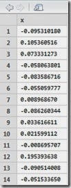
Let’s set our scenario in R and generate the process:

	# Stochastic process stock simulation in R for stock X
	Z <- rnorm(255,0,1) # Random normally distributed values, mean = 0, stdv = 1
	u <- 0.3 # Expected annual return (30%)
	sd <- 0.2 # Expected annual standard deviation (20%)
	s <- 100 # Starting price
	price <- c(s) # Price vector
	a <- 2 # See below
	t <- 1:256 # Time. Days to put on the x axis
	for(i in Z)
	{
	S = s + s*(u/255 + sd/sqrt(255)*i)
	price[a] <- S
	s = S
	a = a + 1
	}
	plot(t,price,main="Time series stock X",xlab="time",ylab="price", type="l",col="blue")
	summary(price)
	statistics<- c(sd(price),mean(price),(price[256]-price[1])/price[1]*100)
	names(statistics) <- c("Volatility","Average price)","Return %")
	print(statistics)

view raw stoch_processes1.R hosted with ❤ by GitHub

Here is the summary of our 256 generated observation:

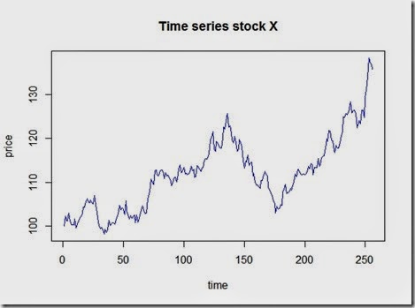
and the plot which looks realistic

Let’s compare this to a pure deterministic model where we assume a constant positive daily return of 30%/255

	h <- 100 #Starting price (equals to s)
	# Projection based on u
	b <- 2
	priceatt <- c(h)
	for(i in t)
	{
	S = h*(1+u/255)
	priceatt[b] <- S
	h = S
	b = b + 1
	}
	length(priceatt)<- length(t)
	# Let's put the points on the graph
	points(t,priceatt)

view raw stoch_processes2.R hosted with ❤ by GitHub

We can clearly see how the stochastic process uses the deterministic model as a base and then implements random shocks in.

Now, let’s have a look at the distributions

	# Frequencies and histograms prices
	boundaries <- seq(from=min(price),to=max(price),by=2)
	boundaries
	# Absolute frequencies
	table(cut(price,boundaries))
	# Relative frequencies
	g<- table(cut(price,boundaries))/sum(table(cut(price,boundaries)))
	plot(g,main="Price distribution")
	# Everything is fine if it sums to 1
	sum(table(cut(price,boundaries))/sum(table(cut(price,boundaries))))
	hist(price,freq=F,col="blue",main="Price frequencies")

view raw stoch_processes3.R hosted with ❤ by GitHub

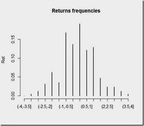
Not that much interesting, not as much as the returns, which we plotted below:

	# Frequencies and histograms daily returns (in percentage)
	c = 2
	rend <- c(0)
	for(i in t)
	{
	r = (price[c] - price[c-1]) / price[c-1]*100
	rend[c] <- r
	c = c + 1
	}
	# Generate class intervals
	limits <- seq(from=-4,to=4,by=0.5)
	limits
	# Absolute frequency
	table(cut(rend,limits))
	# Relative frequency
	table(cut(rend,limits))/sum(table(cut(rend,limits)))
	# Check if it sums to 1
	sum(table(cut(rend,limits))/sum(table(cut(rend,limits))))
	# Plot the histogram
	hist(rend,freq=T,col="blue",main="Returns frequencies")
	# Relative frequency
	Ret<- table(cut(rend,limits))/sum(table(cut(rend,limits)))
	# Plot relative frequency
	plot(Ret,main="Returns frequencies")

view raw stoch_processes4.R hosted with ❤ by GitHub

As you can see, returns are approximately normally distributed, and that’s consistent with our assumptions and the methods we used to simulate the changes in prices. It should be wise to note that drastic changes in prices are rare under these assumptions. However, the stock market proved that “extreme events” occur much more frequently than these models suggests. So, are these models to be thrown away? No, the drawings are nice and look similar to the real ones, but aside from this, I believe these models are an interesting starting point worth future development.

---

Disclaimer
This article is for educational purpose only. The numbers are invented. The author is not responsible for any consequence or loss due to inappropriate use. It may contain mistakes and errors. You should never use this article for purposes different from the educational one.

The maths of Texas Hold ’em with R

Please before continue reading, make sure to read the disclaimer at the bottom of this article.

Every time I watch on tv some game of Texas Hold’em I am always curious about the small percentages which appear in the bottom corners of the screen and tell us the chances of win for each player. There must be some kind of algorithm which implements and refreshes those numbers at each draw.

Today I am going to write about one of the first simulations I put down as code and wrapped my head around. Now that I am a little smarter at coding than I was when I coded this, I believe this whole simulation could be done much better and with A LOT less code… Anyway I guess that is a good sign since the fact I found “mistakes” in my code should mean I improved at least on the very things I made mistakes on.

The code I am about to show estimates the probabilities of drawing a pair, a three of a kind (tris) and a poker.

Let’s proceed, first of all: we need to define the deck and the drawing function.

	# A deck of 52 cards (Jokers are excluded)
	deck = c("A","A","A","A","K","K","K","K","Q","Q","Q","Q","J","J","J","J",10,10,10,10,9,9,9,9,8,8,8,8,7,7,7,7,6,6,6,6,5,5,5,5,4,4,4,4,3,3,3,3,2,2,2,2)
	# This function simulates a hand at Texas Hold'em poker for 2 players and the dealer
	hand <- function()
	{
	player1Hand <- sample(deck,2,F)
	for(i in player1Hand)
	{
	# is.element(i,deck) checks if the element i is in the vector deck
	# match gets the position of the i element in the vector deck and deck[-v] deletes the vth element of the vector deck
	if(is.element(i,deck)
	){
	deck<-deck[-match(i,deck)]
	}
	}
	player2Hand <- sample(deck,2,F)
	for(i in player2Hand)
	{
	if(is.element(i,deck))
	{
	deck<-deck[-match(i,deck)]
	}
	}
	# The flop
	dealt_cards <- sample(deck,3,F)
	for(i in dealt_cards)
	{
	if(is.element(i,deck))
	{
	deck<-deck[-match(i,deck)]
	}
	}
	# The turn
	second_dealt <- sample(deck,1,F)
	for(i in second_dealt)
	{
	if(is.element(i,deck))
	{
	deck<-deck[-match(i,deck)]
	dealt_cards = append(dealt_cards,second_dealt)
	}
	}
	# The river
	third_dealt <- sample(deck,1,F)
	for(i in third_dealt)
	{
	if(is.element(i,deck))
	{
	deck<-deck[-match(i,deck)]
	dealt_cards = append(dealt_cards,third_dealt)
	}
	}
	# Eventually, a list of the results is returned by the function
	results = list(player1Hand,player2Hand,dealt_cards)
	return(results)
	}

view raw texas_holdem_simulation1.R hosted with ❤ by GitHub

Let’s try our drawing function hand() and check the result:

Not that good draw we were looking for huh? Anyway that’s a complete game of Texas Hold’em (provided neither of the two player folded).

Why don’t we create 100 of these games? Here they are:

	# This code builds three arrays where it stores the results of 100 poker hands
	player1Hands <- c(0,0)
	player1 <- matrix(player1Hands,ncol=2)
	player2Hands <- c(0,0)
	player2 <- matrix(player2Hands,ncol=2)
	dealerst <- c(0,0,0,0,0)
	dealer <- matrix(dealerst,ncol=5)
	for(i in 1:100)
	{
	first_round <- hand()
	p1_h <- c(first_round[[1]][1],first_round[[1]][2])
	player1 <- rbind(player1,p1_h)
	p2_h <- c(first_round[[2]][1],first_round[[2]][2])
	player2 <- rbind(player2,p2_h)
	deal_h <- c(first_round[[3]][1],first_round[[3]][2],first_round[[3]][3],first_round[[3]][4],first_round[[3]][5])
	dealer <- rbind(dealer,deal_h)
	}
	player1 <- player1[-1,]
	player2 <- player2[-1,]
	dealer <- dealer[-1,]
	rm(p1_h,p2_h,deal_h,first_round,player1Hands,player2Hands,dealerst,i)

view raw texas_holdem_simulation2.R hosted with ❤ by GitHub

At this stage, if we run the code, R will generate three tables (or matrix) with the results of each one of the 100 simulate games. Something like this:

Now we need only to look for pairs, tris and pokers. We need to define 3 functions as follows:

	# This function runs through all the 100 hands and searches for pairs
	find_pairs <- function()
	{
	pair = 0
	for(i in 1:100)
	{
	if((player1[i,1] == player1[i,2]) | (is.element(player1[i,1],dealer[i,])) | (is.element(player1[i,2],dealer[i,])))
	{
	pair = pair + 1
	}
	}
	return(pair)
	}
	# This function runs through all the 100 hands and searches for tris
	find_tris <- function()
	{
	tris = 0
	for(i in 1:100)
	{
	test = 0
	if((is.element(player1[i,1],dealer[i,]) | is.element(player1[i,2],dealer[i,])) && (player1[i,1] == player1[i,2]))
	{
	tris = tris + 1
	}
	for(b in 2 : 5)
	{
	if(dealer[i,b] == dealer[i,b-1])
	{
	dealer_pair = T
	test = dealer[i,b]
	if(is.element(test,player1[i,]) && dealer_pair)
	{
	tris = tris + 1
	}
	}
	}
	}
	return(tris)
	}
	# This function runs through all the 100 hands and searches for pokers
	find_poker <- function()
	poker = 0
	for(i in 1:100)
	{
	test = 0
	dealer_pair = 0
	test2 = 0
	dealer_tris = 0
	for(b in 2 : 5)
	{
	test = 0
	if(dealer[i,b] == dealer[i,b-1])
	{
	dealer_pair = T
	test = dealer[i,b]
	}else
	{
	dealer_pair = F
	}
	if((player1[i,1] == player1[i,2]) && (dealer_pair) && (player1[i,1] == test))
	{
	poker = poker + 1
	#-------------------
	print(player1[i,])
	print(dealer[i,])
	}
	}
	for(b in 3 : 5)
	{
	test2 = 0
	dealer_tris = 0
	if((dealer[i,b] == dealer[i,b-1]) && (dealer[i,b-1] == dealer[i,b-2]))
	{
	dealer_tris = T
	test2 = dealer[i,b]
	}else
	{
	dealer_tris = F
	}
	if(dealer_tris && ((player1[i,1] == test2) | (player1[i,2] == test2)))
	{
	poker = poker + 1
	#-------------------
	print(player1[i,])
	print(dealer[i,])
	}
	}
	}
	return(poker)
	}
	find_pairs()
	find_tris()
	find_poker()

view raw texas_holdem_simulation3.R hosted with ❤ by GitHub

The result should look like this:

In 100 games, we have got 47 pairs, 2 three of a kind and no pokers! Interesting data! However, this might be a mere case! We need to run this a LOT of times to be sure the odds we obtained are at least near the real ones. Let’s build a function that can do this. For instance, the function below runs n times 100 games and then collect the results. Note that It outputs the probabilities as the mean of the probabilities occurred. Much of the code here is replicated from the functions above. I guess this could have been done a lot better! If you have any idea please let me know or leave a comment!

	# The following function calculates the probabilities of drawing a pair or a tris in a Texas Hold'em game with 2 players and the dealer
	pairs_and_tris <- function(n)
	{
	# This function searches for all the pairs in 100 hands and returns the number of pairs found
	find_pairs <- function()
	{
	pair = 0
	for(i in 1:100){
	if((player1[i,1] == player1[i,2]) | (is.element(player1[i,1],dealer[i,])) | (is.element(player1[i,2],dealer[i,])))
	{
	pair = pair + 1
	}
	}
	return(pair)
	}
	# This function searches for all the tris in 100 hands and returns the number of tris found
	find_tris <- function()
	{
	tris = 0
	for(i in 1:100)
	{
	test = 0
	if((is.element(player1[i,1],dealer[i,]) | is.element(player1[i,2],dealer[i,])) && (player1[i,1] == player1[i,2]))
	{
	tris = tris + 1
	}
	for(b in 2 : 5){
	if(dealer[i,b] == dealer[i,b-1])
	{
	dealer_pair = T
	test = dealer[i,b]
	if(is.element(test,player1[i,]) && dealer_pair)
	{
	tris = tris + 1
	}
	}
	}
	}
	return(tris)
	}
	# This function searches for all the pokers in 100 hands and returns the number of pokers found
	find_poker <- function()
	{
	poker = 0
	for(i in 1:100)
	{
	test = 0
	dealer_pair = 0
	test2 = 0
	dealer_tris = 0
	for(b in 2 : 5)
	{
	test = 0
	if(dealer[i,b] == dealer[i,b-1])
	{
	dealer_pair = T
	test = dealer[i,b]
	}else
	{
	dealer_pair = F
	}
	if((player1[i,1] == player1[i,2]) && (dealer_pair) && (player1[i,1] == test))
	{
	poker = poker + 1
	#-------------------
	print(player1[i,])
	print(dealer[i,])
	}
	}
	for(b in 3 : 5)
	{
	test2 = 0
	dealer_tris = 0
	if((dealer[i,b] == dealer[i,b-1]) && (dealer[i,b-1] == dealer[i,b-2]))
	{
	dealer_tris = T
	test2 = dealer[i,b]
	}else
	{
	dealer_tris = F
	}
	if(dealer_tris && ((player1[i,1] == test2) | (player1[i,2] == test2)))
	{
	poker = poker + 1
	#-------------------
	print(player1[i,])
	print(dealer[i,])
	}
	}
	}
	return(poker)
	}
	# The code below calculates probabilties of pairs and tris for each of the n 100 texas holdem hands simulation
	# The vector help_vector is used to build the matrix risultati_p1 where all the pairs and tris will be stored
	help_vector <- c(0,0,0)
	results_p1 <- matrix(help_vector,ncol=3)
	colnames(results_p1) = c("Pairs per 100 hands","Tris per 100 hands","Poker per 100 hands")
	for(i in 1:n)
	{
	player1Hands <- c(0,0)
	player1 <- matrix(player1Hands,ncol=2)
	player2Hands <- c(0,0)
	player2 <- matrix(player2Hands,ncol=2)
	dealerst <- c(0,0,0,0,0)
	dealer <- matrix(dealerst,ncol=5)
	# The code below simulates 100 texas hold'em hands
	for(i in 1:100)
	{
	first_round <- hand()
	p1_h <- c(first_round[[1]][1],first_round[[1]][2])
	player1 <- rbind(player1,p1_h)
	p2_h <- c(first_round[[2]][1],first_round[[2]][2])
	player2 <- rbind(player2,p2_h)
	deal_h <- c(first_round[[3]][1],first_round[[3]][2],first_round[[3]][3],first_round[[3]][4],first_round[[3]][5])
	dealer <- rbind(dealer,deal_h)
	}
	player1 <- player1[-1,]
	player2 <- player2[-1,]
	dealer <- dealer[-1,]
	pairs <- find_pairs()
	tris <- find_tris()
	#----------------
	poker <- find_poker()
	#----------------
	results__p1 <- c(pairs,tris,poker)
	results_p1 <- rbind(results_p1,results__p1)
	}
	results_p1 <- results_p1[-1,]
	# Results for each 100 hand are shown
	View(results_p1)
	# Final result is printed
	string_to_print <- paste("Given a Texas Hold'em game and two players, here are probabilities for p1 in",n*100,"hands:",sep=" ")
	print(string_to_print)
	# Please note that probabilites are calculated as average of pairs and tris found
	mean_scores = c(mean(results_p1[,1]),mean(results_p1[,2]),mean(results_p1[,3]))
	names(mean_scores) = c("Probability of a pair,","Probability of a tris","Probabilty of a poker")
	return(mean_scores)
	}

view raw texas_holdem_simulation4.R hosted with ❤ by GitHub

Let’s try for instance to run this 10.000 times, with n = 100. Here are the results:

For debugging purposes our function outputs each poker it finds. Since usually pokers are not that frequent it should be fine. 10.000 times seems not to be enough…
Let’s do 100.000 times!!!

This looks better! By simulating in less than 2 minutes 100.000 games of Texas Hold’em with 2 players we concluded that drawing a poker two times in a row is a very unlikely event, drawing a pair is a relative common event while three of a kind is rare, but not as much as poker!

I should mention that, it looks like the probability of a poker is overestimated according to the formal calculation, I believe that is either because it is an “outlier” or because I did not run the simulation a big enough number of times. Anyway the other two probabilities seem fine (you can check for more information on http://en.wikipedia.org/wiki/Poker_probability)

Hope you enjoyed!

---

Disclaimer: This article is for educational purpose ONLY. Odds generated by this code are calculated by a random simulation. As such the odds will represent an approximation of the true odds. They might even be completely wrong or misleading. This code must NOT be used for anything other than educational purpose. The provider of this code does not guarantee the accuracy of the results and accepts no liability for any loss or damage that may occur as a result of the use of this code. Understanding and agreeing to the terms of this disclaimer is a condition of use of this code. By reading the article you confirm you have understood and will comply with this disclaimer.