Wednesday, 30 November 2016

Short circuit currents calculation on high voltage lines

Short circuits are one of the most common failures that can happen when dealing with electrical circuits.

international-symbols---warning-53670-lg

Short circuits can be accidental, think of a tree branch leaning onto a high voltage powerline or due to the breakdown of the isolating material (this is often the case as it gets older and loses its isolating property). Whatever the cause, short circuits are, for sure, an enemy of your electrical systems mainly because the following effects:

Wednesday, 23 November 2016

Solving electrical radial lines with Python

Electrical transmission systems are something we all take for granted. They work in a reliable manner ensuring high quality of service and as few minutes lost per year as possible.

Low voltage lines and most of medium voltage lines are radial lines, that is they are like a branch of a tree with a unique power supply location. Radial lines are relatively easy to work with, you can solve a radial line problem (ie you can get currents and voltages) by applying Boucherot’s theorem to each section of the line. This is a good news for a Python enthusiast as myself, since repetitive tasks lends themselves to be automated with programming.

Since Boucherot’s theorem uses the absolute values of electrical quantities, it is useful when you are working with AC lines and you would like to know the magnitude (rms) of currents and voltages while at the same time you do not really care about the phase differences. The rms values are used, for instance, when you need to choose the protection systems to install and what kind of electrical wires to use.

Suppose you are given the following three phase balanced radial line:

Image 2

You can think of C1, C2 and C3 as industrial motors or any other kind of three phased balanced loads.

Wednesday, 26 October 2016

7th MilanoR meeting + talks live streaming

On 27th of October I’m going to attend the 7th MilanoR meeting featuring the following two talks:

1. Interactive big data analysis with R: SparkR and MongoDB: a friendly walkthrough  by  Thimoty Barbieri and Marco Biglieri

2. Power consumption prediction based on statistical learning techniques by Davide Pandini

This is my first official R event and I’m very much looking forward to it. There has been a strong positive reply from a growing number of people interested in R confirmed by the fact that the tickets were sold out pretty much a few hours after the event was announced.

However, due to this unexpected sudden success in the allocation of the tickets, many people will not be able to attend. Fear not though, the MilanoR staff has just decided to live stream the event on its brand new Facebook page. The event will start around 6.30 PM local time. Feel free to leave a comment and share any thoughts you may have on the topic.

If you would like to know more about the event, the talks and the speakers, check out the following articles:

1. 7th MilanoR Meeting: October 27

2. 7h MilanoR Meeting live on Facebook

Saturday, 24 September 2016

My first Shiny App: control charts

After having carefully followed the online official Shiny tutorial, I decided to make a quick try at making my very first Shiny App. I should say that I found myself very well with the explanation given and Shiny was definitely one of the libraries that took the less time for me to start using it. Of course I’m still not a master of Shiny by no means, but I feel more confident on how to use it and on what can be done with it.

Image 1

I’m working on an R project related to control charts and I was hinted to get to know Shiny, since it is very likely that the project will involve an interactive interface and Shiny fits the bill perfectly for this assignment. For this reason I took an afternoon for getting familiar with Shiny and build this App. Enough talk, let’s get to the App.

Tuesday, 13 September 2016

Some physical considerations on the dynamics of a skydiver

Recently, a friend went skydiving and, me being me, the first thing I could think about was making some physical considerations on his adventure :)

If you think of a falling object, at first you would think of it as falling with a constant acceleration of g. That is, you would neglect air drag. However, if you think of it, air drag is not exactly neglectable when describing the fall of a skydiver. If you neglect air drag, you would get an ever increasing speed which is not at all the case.

Let’s make some physical considerations:

We’ll assume that the only two forces acting on the skydiver are the force of gravity and the air drag. This is the resulting free body diagram:

Image 1


Monday, 12 September 2016

Getting AI smarter with Q-learning: a simple first step in Python

Yesterday I found an “old” script I wrote during a morning in the last semester. I remember being a little bored and interested in the concept of Q-learning. That was about the time Alpha-Go had beaten the world champion of Go and by reading here and there I found out that a bit of Q-learning mixed with deep learning might have been involved.

qlearning[3]

Sunday, 11 September 2016

Building a (reusable?) deep neural network model using Tensorflow

I’ve been experimenting for more than two months with Tensorflow, and while I find it a bit more “low level” if compared to other libraries for machine learning, I like it and hopefully I am getting better at using it. During the learning process I found some minor “obstacles” so I decided to write a short tutorial on how to use this amazing deep learning library.

Friday, 5 August 2016

Image recognition tutorial in R using deep convolutional neural networks (MXNet package)

This is a detailed tutorial on image recognition in R using a deep convolutional neural network provided by the MXNet package. After a short post I wrote some times ago I received a lot of requests and emails for a much more detailed explanation, therefore I decided to write this tutorial. This post will show a reproducible example on how to get 97.5% accuracy score on a faces recognition task in R.

my_convolutional_neural_network

Plain vanilla recurrent neural networks in R: waves prediction

While continuing my study of neural networks and deep learning, I inevitably meet up with recurrent neural networks.

Recurrent neural networks (RNN) are a particular kind of neural networks usually very good at predicting sequences due to their inner working. If your task is to predict a sequence or a periodic signal, then using a RNN might be a good starting point. Plain vanilla RNN work fine but they have a little problem when trying to “keep in memory” events occured, say for instance, more than 20 steps back. The solution to this problem has been addressed with the development of a model called LSTM network. As far as I know, LSTM should usually be preferred to a plain vanilla RNN when possible as it yields better results.

Monday, 25 July 2016

Image recognition in R using convolutional neural networks with the MXNet package

Among R deep learning packages, MXNet is my favourite one. Why you may ask? Well I can’t really say why this time. It feels relatively simple, maybe because at first sight its workflow looks similar to the one used by Keras, maybe because it was my first package for deep learning in R or maybe because it works very good with little effort, who knows.

MXNet is not available on CRAN but it can be easily installed either by using precompiled binaries or by building the package from scratch. I decided to install the GPU version but for some reason my GPU did not want to collaborate so I installed the CPU one that should be fine for what I plan on doing.

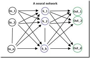
neural_network

As a first experiment with this package, I decided to try and complete some image recognition tasks. However, the first big problem is where to find images to work on, while at the same time not using the same old boring datasets. ImageNet is the correct answer! It provides a collection of URLs to images publicly available that can be downloaded easily using a simple R or Python script.

Sunday, 24 July 2016

Fluid Dynamics: Pressure Drop Modelling [heavily revised]

Some time ago I uploaded a short script on modelling pressure drop in a circular diameter pipe. While at the time I felt I did a good job, I knew there sure was room for improvement. After having attended a (very tough) course on fluid dynamics and applied physics, I feel a lot more confident on this topic and therefore I would like to share a little model I built for a project I am working on.

3d_main_plot

Tuesday, 29 March 2016

How to fit a copula model in R [heavily revised]. Part 2: fitting the copula

Here I am again with part 2. If you would like to read part 1 of this short tutorial on copulas, please click here.

In this second post I am going to select a copula model, fit it to a test dataset, evaluate the fitting and generate random observations from the fitted multivariate distribution. Furthermore I am going to show how to measure correlation using Spearman's Rho and Kendall's Tau. In order to run the code in this post you need the following packages: copula and VineCopula.

The dataset

For this example I am going to use a test dataset. You can download it from this link. This test dataset contains two variables, x and y, characterized by a strong left tail correlation.

By visually inspecting the plot of x versus y you can easily notice that low values of x tends to be highly correlated with low values of y.

Rplot

Sunday, 13 March 2016

How to fit a copula model in R [heavily revised]. Part 1: basic tools


More than a year ago I wrote a short post on how to fit a copula model in R. The post showed how to make a very raw and basic fitting of a test dataset to a two dimensional normal copula (or a gaussian copula if you wish) using the copula package. The content of the post was not much, but that was a big part of what I knew about how to use copulas in R at that time and there was not much documentation available other than the official copula package documentation which is quite technical in my opinion (as it should be) and may not be that easy for a beginner copula user.

Monday, 15 February 2016

Simulating a mass attached to a spring with control theory

Control system theory is very useful when it comes to simulate physical systems and their behaviour.
Suppose you have a mass attached to a spring on an horizontal flat surface. The force diagram associated with this physical system can be sketched as follows:

spring1

By analysing the force diagram, you can actually see that on the x axis the only forces acting on the mass are the elastic force (Fe), the friction (Fr) due to the air resistance and the external force applied to the mass (u). On the y axis the normal force and the force of gravity balance out, therefore there is no motion.


Sunday, 14 February 2016

Solving a circuit with a mutual inductor using LTspice

Mutual inductors can be a lot of fun, and sometimes a bit of an headache if you mess something up or represent them in a complicated way. Take for instance the following circuit designed with Circuit Lab a great online circuit design and simulator tool

circuit

This is one of the first excercises we were taught in our circuit class. As you can probably see, the circuit is composed by two current sources with different frequency, some resistors and a mutual inductor. The aim of the analysis is to find out the total power consumed by the resistors. Let's analyse each problem carefully before proceeding.