Some time ago I uploaded a short script on modelling pressure drop in a circular diameter pipe. While at the time I felt I did a good job, I knew there sure was room for improvement. After having attended a (very tough) course on fluid dynamics and applied physics, I feel a lot more confident on this topic and therefore I would like to share a little model I built for a project I am working on.
I have been asked to make a study for a water pump pumping water out of a reservoir into a storage tank. While working with fluids travelling in pipes, it sometimes is important to account for pressure drop, especially if you need to make yourself an idea of what size of machine you may need. In this case, the parameter to be focused on is the pump’s head.
Let’s make some (hopefully) reasonable assumptions:
- We’ll assume that the pipes have a round constant section and are made of plastics.
- We’ll assume that the flow is stationary. This is a common assumption and usually holds true.
- The fluid used is water so we can reasonably assume it is incompressible.
Under these assumptions, you can break down pressure drop in two components (note that the pressure drop here is measured in meters since these meters will add to the minimum required pump head):
$$Y = \frac{\lambda}{2g} v^2 \frac{L}{D} + \xi \frac{v^2}{2g}$$
The first component is due to friction while the second one is due to turns in the tubes, connections and change of direction of the flow. I’ll be focusing on the first one since the second one is easy to calculate once you know the velocity of the flow and you could easily look up the $\xi$ coefficient depending on the type of tube connection.
As for the first component, we are interested in modelling the pressure drop in meters as a function of the pipe’s diameter and of the volumetric flow rate. We can model the pressure drop for 1 meter of tube, for the sake of simplicity, and then multiply for how many meters we need to use.
So now we need to model $Y_d$ as follows:
$$Y_d = \frac{\lambda}{2g} v^2 \frac{L}{D}$$
Where $L=1$.
First of all we need to find the fluid velocity. Since the fluid is incompressible, it is known that velocity is given by:
$$v = \frac{4 \dot Q}{\pi D^2}$$
where $\dot Q$ is the volumetric flow rate ($\frac{m^3}{s}$) and $D$ is the pipe’s diameter ($m$). The volumetric flow rate is usually a given, since it is usually a project requirement. The pipe diameter is usually not given though.
As far as $\lambda$ is concerned, it is a little bit harder to find this parameter. However, you can usually find it by knowing the Reynold’s number and the rugosity of the tube. As far as the Reynolds number is concerned, it can be calculated using the following formula:
$$Re = \frac{\rho v D}{\mu}$$
while the rugosity of the tube can be looked up according to the material. Next, in order to find $\lambda$ you’d need to use Moody’s Diagram, but since I’m using Python, I can plug in a formula and make a better approximation. Now we have everything, let’s run the simulation!
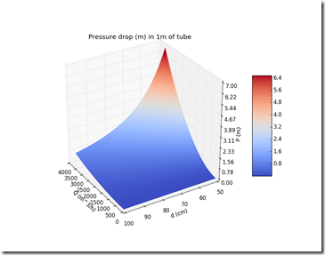
This is the results in a contour plot and two 3D plots.
The contour plot looks sound. As you can see, if at a given pipe’s diameter you keep increasing the flow rate, the pressure drop increases. On the other hand if you keep the flow rate constant and increase the pipe’s diameter, the pressure drop goes down. This seems reasonable and close enough to the expected results. Of course some experiments should be done to assess whether the assumptions hold and if the simulated data matches the measured data.
This is the 3d plot from two different perspectives.
Finally, below is the gist with the code I used to make the plots and run the simulation.
If you have any observation or suggestion, please do comment.


Thanks! ;)
ReplyDeleteVery nice sample.
ReplyDeleteYou say that the pressure drop is in meter. Do you mean meter H2O?
Nice post! This is a very nice blog that I will definitively come back to more times this year! Thanks for informative post. reliable tank line reviews
ReplyDeleteThank you. it was very interesting. I think you should change lbdv(v,d) to lbd(v,d) in line 35.
ReplyDeleteThank you for sharing your helpful code. There is a little typing error in line 35. Correct is pDrop = 0.5 * lbdv(v,d) * v**2 * L / d
ReplyDeleteand not "...* d / L". In your good documentation it is correct.
Nice job sir,I was very much intrested in your work ,can i get a detailed information of the report it will be usefull for me in academics to learn new topics .It would be useful for me if you share this file to my mail.id rahulrao0891@gmail.com
ReplyDelete