Since the first time I was taught the Poisson and Exponential distributions I have been wondering how to apply them to model a real world scenario such as arrivals of people in a shop. Last week I was in a big shopping center and I thought that was the perfect time to gather some data so I chose a shop (randomly) and started recording on a piece of paper how many people arrived and their inter-arrival time.
I went through this process for an hour, in the middle of the afternoon (around 4 to 5pm) during a week day where the influx of customers should be approximately uniform, or so I am told. Here you can download in .txt format, the data I gathered. Note that even though the file is a text file, it is arranged as a .csv so that R can easily detect data.
What is an inter-arrival time? It is the interval of time between each arrival. Assuming that the arrivals are independent, their distribution is exponential. This assumption is further confirmed below by the blue histogram of the observations.
Summary of gathered data:
- I observed the arrival of customer for 58.73 minutes (around an hour)
- During that time 74 “shopping groups” entered the shop. “A shopping group” here is a broad label for a group of 1, 2, 3 or 4 actual customers. The red histograms describes the phenomena in greater detail.
As you can see it seems reasonable to assume that inter-arrival times are exponentially distributed
The red histogram above clearly shows that the majority of “shopping groups” is composed by either a single customer or a couple of customers. Groups of 3 or 4 people are less likely to appear according to the observed data. A good estimate of the probability of the number of people in a shopping group is the relative frequency of the observations.
The following code produces the two plots above
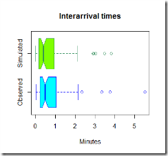
Now that we have uploaded the data, it is time to simulate some observations and compare them to the real one. Below in green is the simulated data.
The code used to simulate the data is here below
Now, the graphs above are pretty, but they are not much use, we need to compare the two sets of graphs to get an idea if our model is fine for this simple task.
It looks like our model tends to overestimate the number of arrivals in the 0-0.5 minutes section, however this is just one simulation and the average arrival time is close to what we expected using this model. It seems reasonable to use this distribution to estimate the inter-arrival times and the number of people arrived in the shop.
The R-code
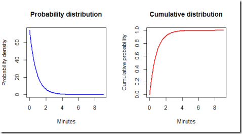
Finally, let's have a look at the ideal exponential distribution given the estimated parameters. Note that some adjustments are necessary because our model is set so that the simulated times are hours, but for practical purposes it is better to work with minutes. Furthermore, by using the exponential distribution formulas we can calculate some probabilities.
By running the code we find out that the probability of the waiting time being less than 3 minutes is 0.975 meaning that it is very likely that one customer group will show up in less than three minutes.
Conclusions.
This model is very basic and simple, both to fit and to run, therefore is very fast to implement. It can be useful to optimize the number of personnel in the store and their function, according to the expected inflow of customers and the average time needed to help the current customers. The hypothesis seem reasonable, given the time of the day considered and provided that the shop does not make some promotion or discount or any other event that could suggest a different behaviour of customers (for instance when there is a discount, it is likely that customers might tell each other to visit the store). For different times of the day, different parameters could be estimated by gathering more data and fitting different exponential distributions.


It shouldn't said this is for beginners only, I have master in math and this was better than the books I'm reading right now (I'm not gonna say what r they :))
ReplyDeleteThat was very flattering! :) Thank you!
DeleteI ran the data provided by you to identify the type of data it exactly is in minitab and it shows it to be 3-Parameter Weibull.
ReplyDeleteGoodness of Fit Test
Distribution AD P LRT P
Normal 3.101 <0.005
Lognormal 0.455 0.262
3-Parameter Lognormal 0.215 * 0.128
Exponential 1.923 0.011
2-Parameter Exponential 1.416 0.032 0.012
Weibull 0.339 >0.250
3-Parameter Weibull 0.272 >0.500 0.132
Smallest Extreme Value 7.958 <0.010
Largest Extreme Value 0.644 0.091
Gamma 0.196 >0.250
3-Parameter Gamma 0.185 * 0.360
Logistic 1.531 <0.005
Loglogistic 0.383 >0.250
3-Parameter Loglogistic 0.319 * 0.578
Hi Amol, thanks for sharing the results!
Deletewhy do you think the results differ, your analysis suggests it to be exponential distribution...
DeleteI've always been taught that inter-arrival times (think of people in a shop or even failures in mechanical components) can, and sometimes are modeled through the use of the exponential distribution. This was a simple attempt at doing that. By taking a look at the histograms of the data, I assumed the distribution was close enough to an exponential and went on from there. I didn't run any goodness of fit test but simply fit the distribution, simulate some data and compared them with the original.
DeleteIf you were to use such model in a real-life context for taking decisions, a more in-depth analysis may be a better option. For instance, your test showed that a Weibull distribution might be a better fit given the data at hand. Using the Weibull (which by the way I think is used in reliability engineering too!) would probably lead to simulated data closer to the real one.