Approximating differential equation with Euler’s method

It looks like it’s time for differential equations.

So, let’s say that you have a differential equation like the one below and you are striving trying to find an analytical solution. Chill out, maybe take a walk outside or ride your bike and calm down: sometimes an analytical solution does not exist. Some differential equations simply don’t have an analytical solution and might drive you mad trying to find it.

Fortunately, there is a method to find the answer you may need, or rather, an approximation of it. This approximation sometimes can be enough of a good answer.

While there are different methods to approximate a solution, I find Euler’s method quite easy to use and implement in Python. Furthermore, this method has just been explained by Sal from Khan Academy in a video on YouTube which is a great explanation in my opinion. You can find it here.

Here below is the differential equation we will be using:

and the solution (in this case it exists)

Here is the Python code algorithm. Note that the smaller the step (h), the better the approximation (although it may take longer).

	# Euler's method for approximating differential equations
	import math
	import matplotlib.pyplot as plt
	# Your differential equation. It should be in the form: dy/dx= f(t,y)
	# Remember that f returns the value of the slope in that point
	def f(t,y):
	return 2-math.e**(-4*t)-2*y
	def solution(t):
	return 1+0.5*math.e**(-4*t)-0.5*math.e**(-2*t)
	t0 = 0
	y0 = 1
	# Step size, the smaller the better, however it may take longer to compute
	h = 0.005
	x = [t0]
	y = [y0]
	y2 = [y0]
	errors = []
	while t0 < 5:
	m = f(t0,y0)
	y1 = y0 + h*m
	t1 = t0+h
	x.append(t1)
	y.append(y1)
	solut = solution(t1)
	y2.append(solut)
	error = abs(y1-solut)/y1*100
	errors.append(error)
	print("Actual t","predicted y","Percentage error %",sep=" ")
	print(t1,y1,error)
	t0=t1
	y0=y1
	print("Mean of error:",sum(errors)/len(errors),"%",sep=" ")
	plt.plot(x,y2,label="Function")
	plt.plot(x,y,label="Approximation")
	plt.legend(loc='upper right')
	plt.title("Euler's method approximation, h="+str(h))
	plt.show()

view raw diff_eq_Euler_approx.py hosted with ❤ by GitHub

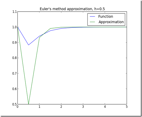
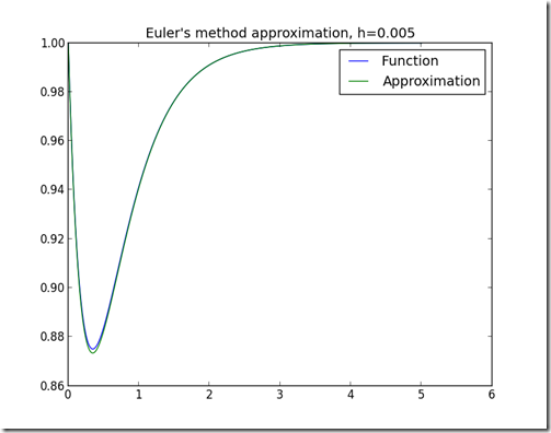
Here are some approximations using different values of h:

Hope this was interesting.

Generate slope fields in R and Python

Here is a short post on how to generate a quick slope field in R and Python.

If you do not know what a slope field is, well I am not the best person to explain it to you since it is a relative new concept for me as well. From what I’ve understood on the subject, a slope field is a graphical way to sort out a first-order differential equation and get a grasp at the solution without having to solve it analytically.

As the Wikipedia’s page says, “it may be used to qualitatively visualize solutions, or to numerically approximate them.”

In general, I feel safe saying that a slope field is some sort of a graphical approach to a differential equation.

Say you have the following differential equation:

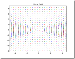
drawing the slope field would look something like this:
In Python (without arrows)

and in R (with arrows, x=f and y=h)

Of course these plots are just very quick and can be improved.

Here is the Python code I used to draw them.

	import numpy as np
	from matplotlib import pyplot as plt
	# Differential equation
	# diff = y'= y/x (or say x+y)
	def diff(x,y):
	return y/x # try also x+y
	x = np.linspace(-10,10,50)
	y = np.linspace(-10,10,50)
	# use x,y
	for j in x:
	for k in y:
	slope = diff(j,k)
	domain = np.linspace(j-0.07,j+0.07,2)
	def fun(x1,y1):
	z = slope*(domain-x1)+y1
	return z
	plt.plot(domain,fun(j,k),solid_capstyle='projecting',solid_joinstyle='bevel')
	plt.title("Slope field y'")
	plt.grid(True)
	plt.show()
	print("End of the program")

view raw slope_field_py.py hosted with ❤ by GitHub

And the R code

	# Our differential equation
	diff <- function(x,y)
	{
	return(x/y) #Try also x+y
	}
	# Line function
	TheLine <- function(x1,y1,slp,d)
	{
	z = slope*(d-x1)+y1
	return(z)
	}
	# Domains
	x = seq(-20,20,0.5)
	y = seq(-20,20,0.5)
	# Points to draw our graph
	f = c(-5,5)
	h = c(-5,5)
	plot(f,h,main="Slope field")
	# Let's generate the slope field
	for(j in x)
	{
	for(k in y)
	{
	slope = diff(j,k)
	domain = seq(j-0.07,j+0.07,0.14)
	z = TheLine(j,k,slope,domain)
	arrows(domain[1],z[1],domain[2],z[2],length=0.08)
	}
	}

view raw slope_field_R.R hosted with ❤ by GitHub

Here is a beautiful slope field for the following differential equation:

In Python

If you need a quick tool for drawing slope fields, this online resource is good, click here.

Hope this was interesting.

Multivariable gradient descent

This article is a follow up of the following:
Gradient descent algorithm

Here below you can find the multivariable, (2 variables version) of the gradient descent algorithm. You could easily add more variables. For sake of simplicity and for making it more intuitive I decided to post the 2 variables case. In fact, it would be quite challenging to plot functions with more than 2 arguments.

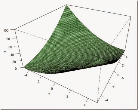
Say you have the function f(x,y) = x**2 + y**2 –2*x*y plotted below (check the bottom of the page for the code to plot the function in R):

Well in this case, we need to calculate two thetas in order to find the point (theta,theta1) such that f(theta,theta1) = minimum.

Here is the simple algorithm in Python to do this:

	from sympy import *
	x = Symbol('x')
	y = Symbol('y')
	z = Symbol('z')
	f = x**2 + y**2 - 2*x*y
	# First partial derivative with respect to x
	fpx = f.diff(x)
	# First partial derivative with respect to y
	fpy = f.diff(y)
	# Gradient
	grad = [fpx,fpy]
	# Data
	theta = 830 #x
	theta1 = 220 #y
	alpha = .01
	iterations = 0
	check = 0
	precision = 1/1000000
	printData = True
	maxIterations = 1000
	while True:
	temptheta = theta - alpha*N(fpx.subs(x,theta).subs(y,theta1)).evalf()
	temptheta1 = theta1 - alpha*N(fpy.subs(y,theta1)).subs(x,theta).evalf()
	#If the number of iterations goes up too much, maybe theta (and/or theta1)
	#is diverging! Let's stop the loop and try to understand.
	iterations += 1
	if iterations > maxIterations:
	print("Too many iterations. Adjust alpha and make sure that the function is convex!")
	printData = False
	break
	#If the value of theta changes less of a certain amount, our goal is met.
	if abs(temptheta-theta) < precision and abs(temptheta1-theta1) < precision:
	break
	#Simultaneous update
	theta = temptheta
	theta1 = temptheta1
	if printData:
	print("The function "+str(f)+" converges to a minimum")
	print("Number of iterations:",iterations,sep=" ")
	print("theta (x0) =",temptheta,sep=" ")
	print("theta1 (y0) =",temptheta1,sep=" ")
	# Output
	#
	# The function x**2 - 2*x*y + y**2 converges to a minimum
	# Number of iterations: 401
	# theta (x0) = 525.000023717248
	# theta1 (y0) = 524.999976282752

view raw multiv_gradient_descent.py hosted with ❤ by GitHub

This function though is really well behaved, in fact, it has a minimum each time x = y. Furthermore, it has not got many different local minimum which could have been a problem. For instance, the function here below would have been harder to deal with.

Finally, note that the function I used in my example is again, convex.
For more information on gradient descent check out the wikipedia page here.
Hope this was useful and interesting.

R code to plot the function

	x <- seq(-5,5,length=100)
	y <- x
	fun <- function(x,y)
	{
	return(x**2+y**2-2*x*y)
	}
	z <- outer(x,y,fun)
	persp(x,y,z,theta=30,phi=30,expand=0.5,col="lightgreen",ltheta=100,xlab="x",ticktype="detailed",ylab="y",zlab="z")

view raw multiv_gradient_descent.R hosted with ❤ by GitHub

Gradient descent algorithm

Today I’m going to post a simple Python implementation of gradient descent, a first-order optimization algorithm. In Machine Learning this technique is pretty useful to find the values of the parameters you need. To do this I will use the module sympy, but you can also do it manually, if you do not have it.

The idea behind it is pretty simple. Imagine you have a function f(x) = x^2 and you want to find the value of x, let’s call it theta, such that f(theta) is the minimum value that f can assume. By iterating the following process a sufficient number of times, you can obtain the desired value of theta:

 

Now, for this method to work, and theta to converge to a value, some conditions must be met, namely:
-The function f must be convex
-The value of alpha must not be too large or too small, since in the first case you’ll end up with the value of theta diverging and in the latter you’ll approach the desired value really slowly
-Depending on the function f, the value of alpha can change significantly.

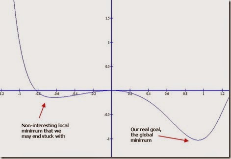
Note that, if the function has local minimums and not just an absolute minimum, this optimization algorithm may well end “trapped” in a local minimum and not find your desired global minimum. For the sake of argument, suppose the function below goes to infinity as x gets bigger and that the global minimum is somewhat near 1. With the algorithm presented here, you may well end up with x = –0.68 or something like that as an answer when you are looking roughly for x = 0.95.

In this case of course, it is trivial to find out the value and you don’t even need derivatives. However, for a different function it may not be that easy, furthermore for multivariable functions it may be even harder (in the next article I will cover multivariable functions).

Here is the Python code of my implementation of the algorithm

	from sympy import *
	import numpy as np
	from matplotlib import pyplot as plt
	x = Symbol('x')
	# Function
	y = x**2
	# First derivative with respect to x
	yprime = y.diff(x)
	# Second derivative with respect to x
	ypp = yprime.diff(x)
	def plotFun():
	space = np.linspace(-5,5,100)
	data = np.array([N(y.subs(x,value)) for value in space])
	plt.plot(space, data)
	plt.show()
	theta = 84
	theta2 = 0
	alpha = .01
	iterations = 0
	check = 0
	precision = 1/1000000
	plot = True
	iterationsMax = 10000
	maxDivergence = 50
	while True:
	theta2 = theta - alpha*N(yprime.subs(x,theta)).evalf()
	iterations += 1
	# If we make too much iterations our program
	# stops and we need to check it to be sure the
	# parameters are correct and it is working properly
	if iterations > iterationsMax:
	print("Too much iterations")
	break
	# Check if theta converges to a value or not
	# We allow a max of 50 divergences
	if theta < theta2:
	print("The value of theta is diverging")
	check += 1
	if check > maxDivergence:
	print("Too much iterations (%s), the value of theta is diverging"%maxDivergence)
	print("Please choose a smaller alpha and, or check that the function is indeed convex")
	plot = False
	break
	# If the value of theta changes less that a certain
	# tolerance, we stop the program since theta has
	# converged to a value.
	if abs(theta - theta2) < precision:
	break
	theta = theta2
	if plot:
	print("Number of iterations:",iterations,"value of theta:",theta2,sep=" ")
	plt.plot(theta,N(y.subs(x,theta)).evalf(),marker='o',color='r')
	plotFun()

view raw gradient_descent.py hosted with ❤ by GitHub

Hope this was interesting and useful.

Generate words through the use of Markov chains

In general, computer programs are believed to be bad at being creative and doing tasks which require “a human mind”. Dealing with the meaning of text, words and sentences is one of these tasks. That’s not always the case. For instance sentiment analysis is a branch of Machine Learning where computer programs try to convey the overall feeling coming from tons of articles.

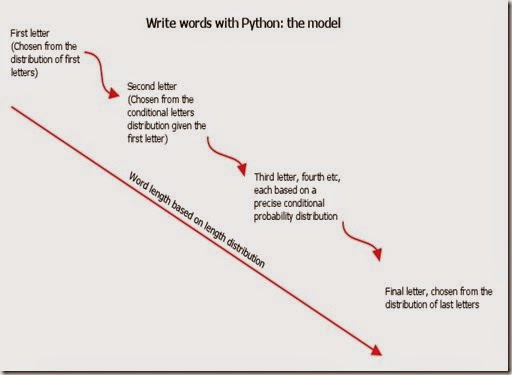
But here we are talking a lot more simpler: by using Markov chains and some statistics, I developed a simple computer program which generates words. The model works as follow:
As a first step, the program is fed with a long text in the selected language. The longer the text, the better. Next, the program analyses each word and gets the probability distributions for the following:
-Length of the word
-First character (or letter)
-Character (or letter) next to a given one
-Last character (or letter)

Then, once gathered all this data, the following function is run in order to generate words:

Each part is then glued together and returned by the function.

On average, 10% of generated words are English (or French, German or Italian) real words or prepositions or some kind of real sequence of characters.

The most interesting aspect, in my opinion, is the fact that by shifting the language of the text fed into the program, one can clearly see how the sequences of characters change dramatically, for instance, by feeding English, the program will be more likely to write “th” in words, by using German words will often contain “ge” and by using Italian words will often end by a vowel.

Here is the code. Note that in order to speed up the word checking process, I had to use the NLTK package which is availably only in Python 2. To avoid the use of Python 2 you could check each word using urllib and an online dictionary by parsing the web page but this way is tediously slow. It would take about 15 minutes to check 1000 words. By using NLTK you can speed up the checking process.

	import numpy as np
	import random
	class ListOperation(object):
	def __init__(self,list1):
	self.list1 = list1
	# This function returns absolute frequencies of
	# occurrence for the characters in listToCheck
	def absFreq(self,listToCheck):
	absFr = []
	for k in listToCheck:
	freq = 0
	for j in self.list1:
	if j == k:
	freq += 1
	absFr.append(freq)
	return absFr
	# This function returns relative frequencies of
	# occurrence for the characters in listToCheck
	def relFreq(self,listToCheck):
	absFreq = self.absFreq(listToCheck)
	relFr = []
	for i in absFreq:
	relFr.append(i/sum(absFreq))
	return relFr
	# This function returns a list of the letters
	# next to the one entered
	def getNext(self,char):
	postChar = []
	for i in self.list1:
	for k in range(len(i)):
	if i[k] == char:
	try:
	postChar.append(i[k+1])
	except:
	postChar.append(" ")
	return postChar
	# This function returns an object of this class
	# containing a list of the first letters in the text
	def getFirstLetters(self):
	firstList = []
	for i in self.list1:
	firstList.append(i[0])
	listF = ListOperation(firstList)
	return listF
	# This function returns an object of this class
	# containing a list of the last letters in the text
	def getLastLetters(self):
	lastLetters = []
	for i in self.list1:
	length = len(i)
	lastLetters.append(i[length-1])
	listU = ListOperation(lastLetters)
	return listU
	# This function returns all the elemets of the list in
	# lower case
	def lowerCase(self):
	listLower = []
	for i in self.list1:
	listLower.append(i.lower())
	return listLower
	# Characters used to build a distribution
	alphabet = ["a","b","c","d","e","f","g","h","i","k","l",\
	"m","n","o","p","q","r","s","t","u","v","w","x","z"]
	# Languages supported
	languages = ["english","italian","french","german"]
	# This function reads data and returns a string
	# you need to load a .txt document containing a
	# sample of the language you selected. The longer
	# the sample, the better word composition.
	def readData(name):
	file = open("C:\\text.txt","r")
	data = file.read()
	file.close()
	return data
	# Text uploaded
	textToCheck = readData("english")
	# The text is splitted
	textToCheckList = textToCheck.split()
	# Create an instance of the class
	textObjectList = ListOperation(textToCheckList)
	#------------------------------------------
	# Let's find all the characters after each one
	# of those in the alphabet list
	postSequences = []
	for letter in alphabet:
	seqPost = textObjectList.getNext(letter)
	postSequences.append(seqPost)
	# For each postSequence we find the absolute frequency
	distAbs = []
	for seq in postSequences:
	distAObject = ListOperation(seq)
	distA = distAObject.absFreq(alphabet)
	distAbs.append(distA)
	# And the relative frequency. However, we
	# must be caareful and delete those which
	# sum up to 0 to avoid exceptions with np
	distRel = []
	for seq in postSequences:
	distRObject = ListOperation(seq)
	if sum(distRObject.absFreq(alphabet)) == 0:
	pass
	print("SOMETHING NOT ADDING TO 1")
	else:
	distR = distRObject.relFreq(alphabet)
	distRel.append(distR)
	#------------------------------------------
	# List of letters at the beginning of a word
	listFirstLetters = ListOperation(textObjectList.getFirstLetters().lowerCase())
	# Distribution of the letter at the beginning of a word
	absFreqFirstLetters = listFirstLetters.absFreq(alphabet)
	relFreqFirstLetters = listFirstLetters.relFreq(alphabet)
	#------------------------------------------
	# List of letters at the end of a word
	listLastLetters = ListOperation(textObjectList.getLastLetters().list1)
	# Distribution of the letter at the end of a word
	absFreqLastLetters = listLastLetters.absFreq(alphabet)
	relFreqLastLetters = listLastLetters.relFreq(alphabet)
	#------------------------------------------
	# This function returns a list containing
	# the length of each word in the string
	def findWordLengDist(string):
	wordList = string.split()
	seqLength = []
	for word in wordList:
	if len(word) <= 18:
	seqLength.append(len(word))
	return seqLength
	# This function returns the probability
	# distribution of the characters in the
	# string used as input
	def generateDist(list1):
	lengthsList = []
	for number in list1:
	if number not in lengthsList:
	lengthsList.append(number)
	lengthsList.sort()
	nLengthsList = []
	for number in lengthsList:
	frequency = 0
	for occurringNumber in list1:
	if number == occurringNumber:
	frequency += 1
	nLengthsList.append(frequency)
	# get relative frequency
	relFreq = []
	for i in nLengthsList:
	relFreq.append(i/sum(nLengthsList))
	# thislist = [lunghezza parole, frequenza relativa]
	dataToReturn = [lengthsList,relFreq]
	# These two should be equal
	if len(lengthsList) != len(relFreq):
	raise ValueError("""The two final lists have diff
	erent length, please check the algorithm""")
	return dataToReturn
	##########################################
	# Word composer function
	##########################################
	# This function outputs strings whose length
	# is similar to the one of the real ones.
	# Also, the structure should be at least similar
	def spitText():
	try:
	word = ""
	# Initial character is chosen based on the
	# distribution (oldChar) of the first
	# characters observed in the text given
	oldChar = np.random.choice(alphabet,replace=True,p=relFreqFirstLetters)
	word = word + oldChar
	for k in range(np.random.choice(distributions[0],replace=True,p=distributions[1])-1):
	newChar = np.random.choice(alphabet,replace=True,p=distRel[alphabet.index(oldChar)])
	word = word + newChar
	oldChar = newChar
	# Same thing for the last character
	lastChar = np.random.choice(alphabet,replace=True,p=relFreqLastLetters)
	word += lastChar
	print(word)
	return word
	except Exception as e:
	print("Exception",e)
	return "0"
	distributions = generateDist(findWordLengDist(textToCheck))
	generatedWords = []
	# Generate 100 words
	for i in range(100):
	word = spitText()
	generatedWords.append(word)
	# And print them out to the screen
	print(generatedWords)
	# Checking existance of words with nltk.corpus
	# and python 2.7. This works only with Python 2
	from nltk.corpus import words
	# Example of word existance checking:
	# True if the word exists, False otherwise
	"word" in words.words()
	# Load words from file
	file = open("C:\\words.txt","r")
	wordsLoaded = file.read().split("\n")
	realWords = []
	for word in wordsLoaded:
	if word in words.words():
	realWords.append(word)
	print(realWords)

view raw words_markov_chain.py hosted with ❤ by GitHub

Hope this was interesting.