Here I am again after a long break!
During my last engineering class I learnt about the frequency response of a system and how this thing can be applied to solve simple problems. But the crucial question from most of us was the following: how would you build such filters, and perhaps more importantly, how would you tune them?
In principle, you could build a simple filter using nothing more than a resistor and a capacitor and, as you might have guessed, LTspice once again comes at rescuing us from our wandering around.
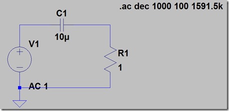
Let’s say we would like to build a simple high pass filter. Then we could try building the following circuit
By applying Kirchhoff current law and then applying the Laplace transform to the equation we can find the transfer function of the system with the following steps:
$$u = Ri + \frac{1}{C} \int \! i(t) \, \mathrm{d}t$$
Then we define $i = x$ and apply the Laplace transform
$$U(s) = RX + \frac{X}{Cs}$$
as a last step we find $x$
$$X(s) = \frac{\frac{s}{R}}{s + \frac{1}{RC}} U(s) = G(s) U(s)$$
where s is a complex variable and $G(s)$ is the transfer function we were looking for.
Matlab can be useful to model control problems since it has a really nice control package. This is the matlab code you need to use in order to simulate the frequency response:
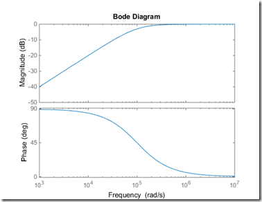
and the output graph we obtain is the following
The horizontal axis in rad/s could be somewhat less intuitive to use. To use frequencies, remember that $w = 2 pi f$ in order to convert between the two.
Let’s try to simulate the very same response using LTspice.
By setting the voltage source AC amplitude to 1V in the voltage source menu and setting the SPICE directive above, we can simulate the frequency response. The SPICE directive that you see near the circuit basically asks LTspice to simulate the frequency response in the 100Hz - 1.6MHz frequency span with a resolution of 1000 points per decade.
By clicking the simulate button we obtain the following graph of the frequency response. Note that the output variable is the current through the resistor (or the voltage on the resistor since we are assuming the resistor is linear and its resistance R is constant).
As you can see from the plot, only signals with a frequency higher than approximately 16kHz can “pass” while the other signals are blocked. How did I find out the approximated cut frequency? By taking a look at the pole of the transfer function one can easily see that there is a pole in $w_0 = 100000$ rad/s, that’s where the approximated bode plot becomes constant. By converting $w_0$ into Hz one can find out the approximated cut frequency. Keep in mind this is a rough approximation though that can be fine for “much” higher or lower frequencies than the cut frequency.
As far as the phase is concerned, low frequency signals experience a phase shift of somewhat less than 90 degrees too, while high frequency experience very low phase shift.


Informative discussion. Many IT professionals are choosing ethical hacker training to build practical skills.
ReplyDelete