How to estimate probability density function from sample data with Python

Suppose you have a sample of your data, maybe even a large sample, and you want to draw some conclusions based on its probability density function. Well, assuming the data is normally distributed, a basic thing to do is to estimate mean and standard deviation, since to fit a normal distribution those two are the only parameters you need.

However, sometimes you might not be that happy with the fitting results. That might be because your sample does not looks exactly bell shaped and you are wondering what would happened if the simulation you ran had taken this fact into account.

For instance, take stock returns, we know they are not normally distributed furthermore there is the “fat tails” problem to take into account. At least it would be interesting estimate a probability density function and then compare it to the parametric pdf you used before.

Here below is a simple example of how I estimated the pdf of a random variable using gaussian_kde from scipy

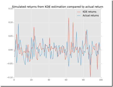
and here is the plot that we get

What we can see is that the estimated pdf is “more dense” around the mean and has some more density on the tails.

Let’s use this data to simulate a sample

For sure in this randomly generated sample there are some extreme values and they look close to the actual sample.

Hope this was interesting and useful.

 

---

Disclaimer
This article is for educational purpose only. The author is not responsible for any consequence or loss due to inappropriate use. The article may well contain mistakes and errors. The numbers used might not be accurate. You should never use this article for purposes different from the educational one.

Image scaling

This is a script that has been resting on my desktop for months. Basically I would like to take my knowledge of image recognition with machine learning a step further and this is a simple step towards that direction.

The basic idea behind the script is to convert the image in a 0 and 1 format which is easier to process with machine learning algorithms. After I wrote the script, I found out there is a function in sklearn that does something similar, anyway I thought I could share the piece of code I wrote, perhaps it could be useful to someone.

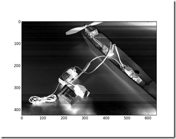
This the image I started with

By using the following script we can convert the image in a more manageable format

This is the result we obtain, A and B respectively

Only numbers between 0 and 1 are used in the picture A above while the picture below uses only 0s and 1.

For sure we loose some information, however this is just a raw script, perhaps I can do better in the future. However, this is a rather complicated image (not to mention the fact that it’s the only sample I have got) the script should yield better results with simpler images and shapes.

Portfolio VaR with Python

After some posts on correlation (How to build a correlation matrix in Python) and variance (How to build a variance-covariance matrix in Python) today I’m posting an example of application: portfolio VaR. Please before you continue reading the article, make sure to read and understand the disclaimer at the bottom of the page. Thank you.

Portfolio VaR is the natural extension of the VaR risk indicator to a portfolio of stocks. The implementation is a little bit harder than the one or the two stock version since it involves calculations with matrices. If you are interested to get a first grasp on VaR you can check my first implementation in R here.

In this script I try to estimate parametric VaR of a portfolio of stocks using historical data.

A brief outline of the process I followed:

1)First I downloaded data from Quandl (they are a great source of free data by the way), then I reshaped the data for each stock into a .csv file to make it resemble the following pattern:

ticker,average return, standard deviation,initial price, R1,R2,R3,…,Rn

where Ri stands for Rth return and initial price is the most recent price.
For my analysis I used simple returns calculation, however it should be more appropriate to use logarithmic returns if possible. Next time I’ll probably be using log returns.

2) The script contains 9 functions:

2 functions are the “builder functions” (fillDicts and runSimulation) and they are used to load the data into the program

2 functions (correlationMatrix and varCovarMatrix) are auxiliary functions since they are used in the VaR function to estimate VaR.

A plot function has been added to plot (if needed) the simulation of future returns by the runSimulation function. The model used to simulate future prices is fairly simple and can be found here.

A function (portfolioExpectedReturn) to calculate portfolio expected returns based on historical data

And finally, two functions (simple_optimise_return and optimise_risk_return) to optimise the portfolio for high returns and the risk/return ratio, respectively.

3)Some preliminary notes and some assumptions.
The model is based on parametric VaR, therefore it is assuming that returns are normally distributed like a smooth Bell curve. Furthermore, the VaR is calculated for an holding period of 1 day.

For the sake of simplicity I calculated 99% VaR for each example and ran the optimisation functions for a portfolio of 10 stocks. The optimisation functions operate as follow:

simple_optimise_return yields a portfolio of n stocks with the highest average daily return in the sample while optimise_risk_return yields the 10 stocks with higher average return to standard deviation ratio. The idea behind the second optimisation is that you may want to get the highest return possible for unit of risk that you are bearing. Note that I am assuming that the total invested amount is equally distributed among the 10 stocks (10%  of the total amount is invested in each stock).

While keeping in mind that the past usually does not predict with great accuracy the future, this script let me grasp an insight of what could have (possibly) been a good portfolio of stocks in the last years.

A sidenote: since this is just for fun, some data is actually missing and some stocks have longer time series since they were on the market long before than others.

Another sidenote: a great improvement to this script could be the calculation of the advantages (in terms of less risk) of diversification and optimisation for correlation (maximum and minimum correlation for instance)

Now I run the program

And after some computations here is the result that we get:

The results look interesting to me, especially since the VaR of the last portfolio is really low if compared with the first portfolio I used to test the VaR function and the non-weighted return seems pretty good too.

---

Disclaimer
This article is for educational purpose only. The author is not responsible for any consequence or loss due to inappropriate use. The article may well contain mistakes and errors. The numbers used might not be accurate. You should never use this article for purposes different from the educational one.

How to build a variance-covariance matrix in Python

Recently I wrote a script to calculate the VaR of a portfolio of stocks given historical prices and returns and, in order to do that, I had to study the basics of a variance-covariance matrix.

First of all, what is it?
The formal definition should sound something like this: a variance-covariance matrix is a matrix whose element in the i,j position is the covariance between the ith and jth elements of a vector of random variables. Informally, we may say that a variance-covariance matrix is the matrix of the covariances and since the covariance of a random variable with itself is its variance, the main diagonal of the matrix is filled with the variances of the random variables (hence the fancy name).

What is it useful for?
When calculating VaR, say for a single stock, you need to gather the standard deviation of the returns of your stock. However, when calculating the VaR of a portfolio, things get pretty messy pretty quick, since you cannot simply add or subtract variances. In a more intuitive way, we may say that the variance-covariance matrix generalizes the notion of variance to multiple dimensions.

So how can we build it in Python?
Here is a simple template of how I built mine. I used only two stocks, but in the script I talked about earlier I used 500 stocks, you can easily imagine what a mess it can be if you miss some numbers.

Before showing the code, let’s take a quick look at relationships between variance, standard deviation and covariance:

Standard deviation is the square root of the variance

Covariance can be obtained given correlation (check how to build a correlation matrix) and standard deviations.

Now we can look at the script:

And here is the output:

Hope this was interesting.

How to build a correlation matrix in Python

Suppose you have an array of data, stocks returns for instance, and you are wondering whether there is some degree of correlation. If you are using Python then it is easy to plug in your data and do some simple calculations.

Here is a simple example of a correlation matrix using Python. This matrix shows the correlation between 10 variables (10x10 matrix): as you can see, the correlation of a variable with itself is 1 as expected.

By entering more variables into the calculation the matrix becomes more difficult to interpret although it remains quite nice to visualize. Here below is an example of a 50x50 matrix.

The code I used is really simple, you can find it here below. Basically I built a random array with 10/50 data points and then used the numpy function “corrcoef” which handles all the troubles of building a matrix in an elegant way.

Some plots with matplotlib

I recently updated matplotlib and could finally use the style attribute from the updated module. I thought it might be a good time to plot some data and try it out.

In order to get a grasp on how some emerging markets have performed so far, I thought I could plot some data on the real GDP (GDP adjusted for inflation) and perhaps compare it to a big part of the EU’s economy (Germany).

The data I used is from Quandl a great source of data you should check it out https://www.quandl.com/

Note: dotted lines indicates that the data is prospective (in this case obtained through linear regression).

Hope this was interesting

Handwritten number recognition with Python (Machine Learning)

Here I am again with Machine Learning! This time I’ve achieved a great result though (for me at least!). By using another great dataset from UCI I was able to write a decent ML script which scored 95% in the testing part! I am really satisfied with the result.

Here is a sample of what the script should be able to read (in the example the number 9):

Some numbers, as the one above, were clear, others not so clear, since they were handwritten and then somehow (I do not know how) converted into digital images.

I had a hard time figuring out how the attributes in the dataset were coded but in the end I managed to figure it out! I guess making up such a dataset was a really long and boring work.

Anyway here is my script and below you can find the result of the test on the last 50 numbers or so.

This time I got 89% success rate! Pretty good I guess! I wonder whether I could train Python to recognize other things, maybe faces or other! Well first of all I have to figure out how to convert a picture into readable numpy arrays. Readable for Python of course!! If you have any suggestion please do leave a comment!

Here below is the citation of the source where I found the dataset “Semeion Handwritten Digits Data Set”:

Bache, K. & Lichman, M. (2013). UCI Machine Learning Repository [http://archive.ics.uci.edu/ml]. Irvine, CA: University of California, School of Information and Computer Science.

and

Semeion Research Center of Sciences of Communication, via Sersale 117, 00128 Rome, Italy
Tattile Via Gaetano Donizetti, 1-3-5,25030 Mairano (Brescia), Italy.

 

Hope this was interesting!

Poker hands recognition (Machine Learning)

A few months ago I downloaded the scikit-learn package for Python, for those of you who might not be aware, scikit-learn is a powerful yet very simple package useful to apply machine learning. Basically they give you “all” the algorithms you may need and you “only” have to get the data and make it ready to feed into the scikit-learn algorithm.

Anyway, I only recently had time to check it out and write some code, furthermore only recently I found a great site full of sample datasets dedicated to machine learning (check it out here). Since the data from this great site is more or less in the right shape for being ready to import (.txt files or similar) the only task left to the programmer is to put it into numpy arrays.

This is one of my first attempt at generating a “real” machine learning program.

I won’t post the pre-settings script since it is pretty boring, instead I’ll briefly describe the pre-setting: basically, using a simple script I’ve splitted the training samples from the database in two .txt files trainingP.txt and target.txt respectively. TrainingP.txt contains the questions (the hands of poker) and target.txt contains the answers (=the score, that’s to say poker, full house etc… coded into numbers according to the description given in the database description file).

Below is the ml script: it is composed of 3 parts: setting, training and testing

setting: import the training sets and fit them into numpy arrays of the correct shape

training: fit the data into the model using scikit-learn

testing: test the algorithm and check what it has learned so far! Some statistics are printed, for reference. Check the results below!

So far the best score is 56.4%, I wonder if I did everything correctly! Anyway soon I will post a script with better results and achievements!

Below is the citation of the source of the database, according to their citation policy.

The name of the dataset is Poker Hand and it is from:

Bache, K. & Lichman, M. (2013). UCI Machine Learning Repository[http://archive.ics.uci.edu/ml]. Irvine, CA: University of California, School of Information and Computer Science.

Fluid dynamics: pressure drop modelling

Likely the last post of the year, on a rather intriguing subject: fluid dynamics.

Recently I’ve been asked to model a simulation for a series of pipes through which water flows out of a reservoir. The task seems quite easy at first, however many factors must be taken into account. Pressure drop due to friction is one of the things that need to be addressed. Therefore, I documented myself a little on the subject and developed a simple model to take friction into account. Pressure drop depends both by the speed of the water and the pipes diameter.

Here is a short piece of code to calculate pressure drop. Note that we are using the average speed of the water. For each average speed we can draw a line that shows the pressure drop versus the pipe’s diameter.

Considering the fact that this was my first attempt I think the results are pretty good when compared with an actual diagram such as this (note that on this graph you’ll need to multiply pressure drop by 10 to compare pears to pears and apples to apples):

Here is the code I used. I should mention, I had a hard time finding out how to do this and furthermore I couldn’t find a comprehensive piece lecture where fluid dynamics is analysed in depth. Online there is a lot of material on Bernoulli’s equation and Torricelli’s special case but it is definitely harder to find out how to model real fluids, friction and fluid dynamics in general. Hope someone will upload some good material.

And here comes the whole Solar System! ;)

Modelling Sun, Earth and Moon only? Naah that’s too naive. Let’s add some other planets!
The code on my previous article was rather ugly. It did not follow an OOP style and it was mostly non re-usable. Aside from the content of the piece of code I posted in this article, I’m quite satisfied with how I set it: a class for planets and a class to handle time. Sure, perhaps this is not the smartest way of using a class, however for someone like me, who programs mainly as a hobby, that’s fine I guess.
This piece of code models and simulates the whole Solar System (without the Sun, you can add it though!) and gives you, aside from the code, a hint on how slow/fast planets are orbiting around the Sun. note that I use large intervals of time (10000 seconds or similar). This model for sure can be improved. For instance the colours could be improved and, jokes aside, perhaps elliptical orbits could be implemented instead of circular. To do that I still need to work on my knowledge of gravity and its implementation in Python.


Anyway I’ll keep you posted. That’s it for now, here’s the code of the model and the YouTube video I made (but couldn’t load in the post, not sure why)

[EDIT]: I've finally made it and load the video here too! Enjoy

Earth Moon system orbiting around the Sun and VPython

Hello everyone! A few days ago my friend, as a joke, bet me to reproduce the Moon orbiting around the Earth. Well, I was a little afraid the model could be a little slow using matplotlib and its animation functions. Fortunately I found out VPython, a great 3D package: click here to get to their homepage. VPython, in my opinion, provides one of the simplest yet most brilliant package for 3D graphics. It’s shockingly easy to learn: it took less than an hour for me to learn the basics and start doing something interesting. Furthermore if you’re used to vectors and working with them, VPython provides simple functions for vectors calculations.

Check the model below (Earth and Moon orbiting around the Sun). I also made a video:

Hope this was entertaining! Next comes the whole Solar System!

Gini coefficient, concentration measurement: an implementation in R

Another subject we took in the statistics class was the Gini index.

Gini index or ratio or coefficient is used to calculate how much a certain transferable phenomenon such as income or stocks for instance, is concentrated.

For example, say you are evaluating a company and you’d like to know more about how the shares are divided among the shareholders. You could use Gini index for that!

I’ve calculated the index using R and random data you can download here. In case you’d like to know more about Gini index check here.

Here my simple R implementation of the index.

Here below are the results

It looks like the data I used shows a 24% concentration. Cool!

Pearson’s chi-squared test: a simple implementation in R (test of independence)

Hi everyone! Today I found my old statistics workbooks and start wondering what I could get out of them.

Statistics can look pretty boring when using only pen and paper, since many times you’re just making a lot of repetitive calculations. However, the results of those calculations might of course be interesting.

Person’s chi-squared test is a simple test, as my professor put it, one of the first tests you should be performing when analysing a double entry table. You might be asking yourself why. Well, the answer is that this test looks for connection between the two variables in the table. As you might know connection is different from dependence. Dependence is of course a stronger bond and kind of a “one way bond” whilst connection is sort of a “double way bond”. If there’s no or little connection, then you might want to change variables in play since there is nothing but little interest in performing further tests on the same set of data.

Check on Wikipedia for more information on the theory.

Here is the R code I used to implement the test on the raw data at the bottom of the page.

Below is the output, it seems there’s a feeble connection between the two phenomena we studied.

The data I used for the simulation are available to be downloaded here.

Here again Java

Java, Java and Java again! Here is my last script in Java, which I wrote today.

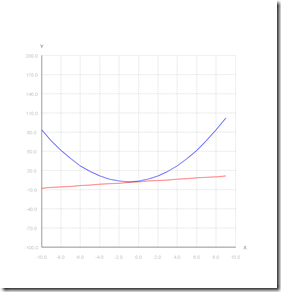
The script is quite simple, it is composed of three classes and lets you handle some basic calculations with lines and parabolas on the real plane and calculate the area under the curve (definite integrals).

Optionally you can plot the data.

Here is the main class with a simple example:

And the integral class which handles all the background operations

Optionally, should you want to output something to a .txt file, here is the class that can help in doing that:

Bye until the next project!

Java again, in English this time though! ;)

As i said earlier in my article in German, I studied Java only once in a while, since I had so many other things to do and study. Anyway here is another bit of code I’ve written in order to practice what I’ve learnt.

This script is a simple program to keep track of your inventory. Frankly speaking, an excel spreadsheet would have been faster and easier but where’s the fun in it?

There are three classes: the main class, the products class and the inventory class. In the products class lies all the code related to the object “product” while in the inventory class you can find all the code needed to run the inventory. Finally the main class executes the main program and (as it should be I guess).

For the sole purpose of exercising myself with Java, I tried to generate a inventory of food with three items. However you can easily add as many inventories as you like and figure out a way to speed up the process of adding items to each inventory.

Perhaps in the future I’ll add the option to print out a bar chart or something similar as soon as I have time to study Java. As for now, I find it quite interesting and demanding since it asks every time for the type of the data you are going to work with and the arrays are different from python’s lists. That can be a small issue for someone who got used to Python as myself. Furthermore Java libraries are hugely vast and that can be overwhelming at the beginning. Nonetheless I hope to get better at it soon!

Here is the products class

public class Products 
{
	private String name;
	private int id;
	private int quantity;
	private double price;
	
	//Constructor of the class
	public Products(String name,int id, int quantity, double d)
	{
		this.name = name;
		this.id = id;
		this.quantity = quantity;
		this.price = d;
	}
	
	//Quantity setter and update method
	public void changeQuantity(int q,String s)
	{
		if(s.equals("add"))
		{
			this.quantity += q;
		}else if(s.equals("subtract"))
		{
			this.quantity -= q;
		}
		System.out.println("Warehouse stock updated succesfully!");
	}
	
	//Price setter
	public void changePrice(double p)
	{
		this.price = p;
		System.out.println("Price changed succesfully!");
	}
	
	//Get all the info on the product
	public void getInfoProduct()
	{
		System.out.println("As for product "+this.name+" with id: "+this.id);
		System.out.println("Quantity available: "+this.quantity);
		System.out.println("Price "+this.price);
		System.out.println("Total value in stock: " + this.getTotalValue());
	}
	
	//This function returns the total value of the stock for the product
	public double getTotalValue()
	{
		double totalValue = this.price*this.quantity;
		return totalValue;
	}
	
}

The main class

public class mainClass 
{

	public static void main(String[] args) 
	{	
		//we create the products
		Products bread = new Products("Bread",0,10,0.5);
		Products ooil = new Products("Olive oil",1,20,4.00);
		Products oranges = new Products("Oranges",2,5,2.50);
		
		//we create the inventory and add products to it
		Inventory inventory1 = new Inventory("Inventory 1");
		inventory1.addProduct(bread);
		inventory1.addProduct(ooil);
		inventory1.addProduct(oranges);
		
		//We print info on the products
		bread.getInfoProduct();
		ooil.getInfoProduct();
		oranges.getInfoProduct();
		
		//And the total value of the inventory
		System.out.println("\nTotal value of the inventory is "+inventory1.getInventoryValue());
	}
}

Finally, the inventory class

//Dynamics arrays. I found them similar to those in Python
import java.util.ArrayList;
import java.util.List;

public class Inventory 
{
	private String name;
	//Products[] productsInStock = new Products[]{};
	List<Products> productsInStock = new ArrayList<Products>();
	private int totalItems = 0;
	
	//Constructor of the class
	public Inventory(String name)
	{
		this.name = name;
	}	
	
	//Add a product object to the inventory array
	public void addProduct(Products p)
	{
		productsInStock.add(p);
		this.totalItems += 1;
		System.out.println("Product added to inventory "+this.name+" succesfully!");
	}
	
	//Get the total value of the inventory
	public double getInventoryValue()
	{
		double valueToReturn=0;
		int lenAr = this.totalItems;
		for(int i=0;i<lenAr;i++)
		{
			valueToReturn += this.productsInStock.get(i).getTotalValue();
		}
		return valueToReturn;
	}
}

Here below is the output

Product added to inventory Inventory 1 succesfully!
Product added to inventory Inventory 1 succesfully!
Product added to inventory Inventory 1 succesfully!
As for product Bread with id: 0
Quantity available: 10
Price 0.5
Total value in stock: 5.0
As for product Olive oil with id: 1
Quantity available: 20
Price 4.0
Total value in stock: 80.0
As for product Oranges with id: 2
Quantity available: 5
Price 2.5
Total value in stock: 12.5

Total value of the inventory is 97.5

Hope this was interesting.