The Fourier transform is surely one of the most amazing pieces of maths applied to the sciences. For starters it is defined as follows:
The definition is fine provided that you can take the integral of u(x) over R. (Technically you should say that u(x) belongs to L1(R). But aside from these technicalities, how awesome is that definition? Calculating the FT of a function with pen and paper isn’t that straight forward at all, except in some cases. It involves mainly using complex analysis techniques. If you are familiar with calculating “standard integrals” it is rare that you can apply the same techniques here.
But how can we apply this to something? Well it turns out that if you have a signal u(x) in the time domain, its Fourier transform is the signal representation in the frequency domain. Essentially the FT enables you to decompose your time domain signal into all the frequencies that make up that signal. A first simple application is deleting noise from a signal. By checking the signal spectrum (its FT) you can choose which frequencies you need to delete from the signal in order to remove the noise. Then you just apply the inverse FT and get back your time domain signal cleaned up (more or less). Now obviously the math behind this is hairy, however this should not scare you at all, and if you are interested in these subjects I suggest you to check out some resources to get a better grasp of how all of this works.
In order to compute the FT of a signal with Python we need to use the ftt function built in into Scipy. FTT stands for Fast Fourier Transform and it is a brilliant algorithm to speed up the otherwise very long calculation of the FT of a real signal.
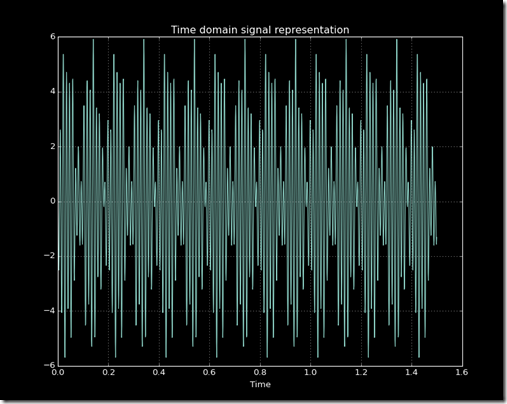
The signal I’ve made is a linear combination of the sine and cosine function, pretty straightforward here is its representation in the time domain:
A closer look to our signal:
Now by taking the FFT we get a list of complex numbers. Then we take the absolute value of those numbers and plot them to represent the spectrum:
Eventually, we just need to fix the lower axis and switch from bins to Hz. Since the plot is symmetrical we can take out the right half without losing information. As you can see below, we have three spikes in the frequency domain. Those three peaks corresponds to the three frequencies we set earlier in the signal (85,50,75 Hz).
Hope you enjoyed this, soon I’ll make a post about applying this to a real signal, such as the recording of guitar notes. Below is the code I used to plot the data above. Have fun!


No comments:
Post a Comment