Simulations can be useful in an unimaginably large number of scenarios. Finance in particular is a field of study where maths and statistics have made led to great advances (sometimes for the good, sometimes for the bad). Value at Risk is just another example of subject where a simulation approach could be handy.
But, what is VaR? VaR is an indicator used in risk management, it represents the maximum potential loss which can occur to a portfolio of a certain investor, say 95% of the times. Well, actually, it could be better to say that 5% of the times the loss will be larger than what VaR predicted (and it could be way larger). In this case we say that we are calculating VaR with 5% confidence.
There are at least three ways of calculating VaR:
-Parametric VaR
-Historical VaR
-Monte Carlo VaR
Let’s see each of them. For simplicity we will assume that our hypothetical investor has only one type of stock in their portfolio and that the holding period N is equal to 1.
Parametric VaR: Here is the formula
Where W0 is the value of the portfolio at time of calculation, N is the holding period, sigma is the daily volatility and Z is the inverse of the normal distribution for 1 minus alpha which is the confidence level. (If alpha is 5% then Z is approximately –1.64, note however that VaR is a positive quantity). The use of the normal distribution of course hides important assumptions which often are fundamental for the reliability of these methods.
HR are the historical returns and Percentile is the quantile function in R applied to the historical returns. Note that there is no square root of N, since the holding period is equal to 1. If holding period > 1 day you should multiply this for N as above.
Monte Carlo VaR:
With this approach you simulate a stochastic process which represent the path of the stock and then once you have calculated the logarithmic returns you just check the 5% percentile return and multiply it for the value of the portfolio at time 0.
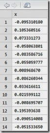
Let’s see how to implement all this in R. The data used has been invented, and is downloadable from here
Here are some results:
The results tells us that our investor should experience losses greater than 2835.56 (or 1843.85) only 5% of the times. Usually this two values should not differ that much, however, considering how they are structured and that the data I used is completely made up and too short for historical VaR, it is still fine that we got these results. Usually the time series from which data is gathered are very long, the longer the series the more precise the result. In the last version of VaR, once simulated the behaviour of the stock you just calculate the logarithmic returns and then take out the 95% percentile.
For more information, check the wikipedia page here.
Disclaimer
This article is for educational purpose only. The numbers are invented. The author is not responsible for any consequence or loss due to inappropriate use. It can contain mistakes and errors. You should never use this article for purposes different from the educational one.


I believe that in calculating historical VaR and if holding period is >1 you mean multiplying by the square root of N and not just N. Or it is the same as with when calculating parametric VaR and holding period>1.
ReplyDeleteCheers.
austine88
ReplyDeletelink austine88
link alternatif austine88
Bandar online slot dan togel
agen slot terlengkap
slot gacor
situs judi online
bandar togel
slot online terbaik
agen slot dan togel
situs togel dan slot
togel singapore
slot online terpercaya
agen slot
Pragmatic Play
Deposit pulsa
Deposit pulsa
livegames casino