Step response of a RLC series circuit

Today I am going to make a brief description of the step response of a RLC series circuit. This is the schematic made with LTspice

As you can see the components used are a resistor, an inductor and a capacitor connected in series. By applying Kirchhoff voltage law we obtain the following equation

$$u(t) = R x(t) + L\frac{dx(t)}{dt} + \frac{1}{C} \int x(t)dt $$

Three-phase symmetric perfectly balanced system LTspice simulation

A symmetric, three-phase and perfectly balanced system can be easily modelled either by pen and paper with the use of phasors or using LTspice which is faster. In case you would like to try I suggest to first try the pen and paper way and then check the results on the simulator. A basic example of such system would be the following:

How to simulate a simple high pass filters on LTspice

Here I am again after a long break!

During my last engineering class I learnt about the frequency response of a system and how this thing can be applied to solve simple problems. But the crucial question from most of us was the following: how would you build such filters, and perhaps more importantly, how would you tune them?

In principle, you could build a simple filter using nothing more than a resistor and a capacitor and, as you might have guessed, LTspice once again comes at rescuing us from our wandering around.

Let’s say we would like to build a simple high pass filter. Then we could try building the following circuit

Selecting the number of neurons in the hidden layer of a neural network

Recently I wrote a post for DataScience+ (which by the way is a great website for learning about R) explaining how to fit a neural network in R using the neuralnet package, however I glossed over the “how to choose the number of neurons in the hidden layer” part. The glossing over is mainly due to the fact that there is no fixed rule or suggested “best” rule for this task but the mainstream approach (as far as I know) is mostly a trial and error process starting from a set of rules of thumb and a heavy cross validating attitude.

Predicting creditability using logistic regression in R: cross validating the classifier (part 2)

Now that we fitted the classifier and run some preliminary tests, in order to get a grasp at how our model is doing when predicting creditability we need to run some cross validation methods.
Cross validation is a model evaluation method that does not use conventional fitting measures (such as R^2 of linear regression) when trying to evaluate the model. Cross validation is focused on the predictive ability of the model. The process it follows is the following: the dataset is splitted in a training and testing set, the model is trained on the testing set and tested on the test set.

Note that running this process one time gives you a somewhat unreliable estimate of the performance of your model since this estimate usually has a non-neglectable variance.

Predicting creditability using logistic regression in R (part 1)

As I said in the previous post, this summer I’ve been learning some of the most popular machine learning algorithms and trying to apply what I’ve learned to real world scenarios. The German Credit dataset provided by the UCI Machine Learning Repository is another great example of application.

The German Credit dataset contains 1000 samples of applicants asking for some kind of loan and the creditability (either good or bad)  alongside with 20 features that are believed to be relevant in predicting creditability. Some examples are: the duration of the loan, the amount, the age of the applicant, the sex, and so on. Note that the dataset contains both categorical and quantitative features.
This is a classical example of a binary classification task, where our goal is essentially to build a model that can improve the selection process of the applicants.

RandomForestClassifier on the cars dataset ML

Since the beginning of this summer I have been practicing a lot with Scikit-learn to improve my knowledge of Machine Learning both on theory and practice. Last week I also tried to tackle some of the Kaggle competitions although they are really tough if you wish to get into the top 50 best scores. Perhaps I will post something about the experience in the future.

Scikit-learn is a (almost) ready to use package for Machine Learning in Python. It is so very user friendly and in some cases not that much coding around is needed to achieve interesting results such as in the case of the cars dataset.

The cars dataset, from the UCI Machine Learning Repository, is a collection of about 1700 entries of cars each with 6 features that can be easily recognized by the name (buying, maint, doors, persons, lug_boot, safety). Check the dataset description for more detailed information. The feature to be predicted is “class” and the possible values are unacc,acc,good,v-good. Most of the features are categorical, therefore they need to be encoded into numbers. Pandas is great for quick features encoding.

Using Arduino to measure friction coefficient

As a sideproject I decided to design a simple experiment and use Arduino to measure the friction coefficient of an object sliding on a given material.

Ideally we would like our first object to slide (not roll) on a sheet of a given material as below:

If we know the angle (we can easily set it) and the mass of the wooden block, then the only unknown variable is the friction coefficient and we can easily estimate it by measuring how long it took for the block to go over a certain distance x.

European Option Pricing with Python, Java and C++

Please make sure to read the disclaimer at the bottom of the page before continuing reading.

Plain vanilla call and put european options are one of the simplest financial derivatives existing. A european call (put) option is essentially a contract which by paying a fee gives you the right to buy (sell) a stock at a predetermined price, the strike price, at a future date. This kind of contracts was originally intended as an insurance tool for companies to fix the selling price of their goods and hedge the price risk.

Options have some interesting features, for starters, if you are the buyer of an option the payoff is potentially unlimited and the loss is limited to the option price as you can see by the payoff diagram below

of course the reverse is true for the seller (huge downside and limited upside).

Controlling lights according to sunlight using only few electronic components

At the beginning of this summer, I was asked to provide a simple (and possibly cost-effective) solution to a simple problem: how can I do in order for my garden LED lights to turn themselves on and off according to the sunlight?

There are plenty of ready to use circuits and tools that one can use to answer this question, however I decided to try and design something “new” empowered by what I recently learned about NPN transistors, relays and LT-Spice IV. Let me talk you through my workflow:

The problem and the setting:

The LED lights which provide illumination in the garden are powered by a solar panel which during the day charges the battery. At night, the stored energy is used to power the lamp. The solar charge controller ensures that the charging process is smooth and that everything is going as it should during the charge and discharge processes. Since the solar charge controller is very minimal, it does not have a timer or a switch to turn on and off the lights. A manual switch is therefore used instead (not shown in the picture and to be replaced by this project). The lamp is a 12V 4.5W LED lamp.

The solution

Basic Hidden Markov model

A hidden Markov model is a statistical model which builds upon the concept of a Markov chain.

The idea behind the model is simple: imagine your system can be modeled as a Markov chain and the signals emitted by the system depend only on the current state of the system. If the states of the system are not visible and what you can observe are only the emitted signals, then this is a Hidden Markov model.

Simple regression models in R

Linear regression models are one the simplest and yet a very powerful models you can use in R to fit observed data and try to predict quantitative phenomena.

Say you know that a certain variable y is somewhat correlated with a certain variable x and you can reasonably get an idea of what y would be given x. A class example is the price of houses (y) and square meters (x). It is reasonable to assume that, within a certain range and given the same location, square meters are correlated with the price of the house. As a first rough approximation one could try out the hypothesis that price is directly proportional to square meters.

Now what if you would like to predict the possible price of a flat of 80 square meters? Well, an initial approach could be gathering the data of houses in the same location and with similar characteristics and then fit a model.

A linear model with one predicting variable might be the following:

Alpha and Beta can be found by looking for for the two values that minimise the error of the model relative to the observed data. Basically the procedure of finding the two coefficient is equivalent to finding the “closest” line to our data. Of course this will still be an estimate and it will probably not match any of the observed values.

Estimating arrival times of people in a shop using R

Since the first time I was taught the Poisson and Exponential distributions I have been wondering how to apply them to model a real world scenario such as arrivals of people in a shop. Last week I was in a big shopping center and I thought that was the perfect time to gather some data so I chose a shop (randomly) and started recording on a piece of paper how many people arrived and their inter-arrival time.

I went through this process for an hour, in the middle of the afternoon (around 4 to 5pm) during a week day where the influx of customers should be approximately uniform, or so I am told. Here you can download in .txt format, the data I gathered. Note that even though the file is a text file, it is arranged as a .csv so that R can easily detect data.

What is an inter-arrival time? It is the interval of time between each arrival. Assuming that the arrivals are independent, their distribution is exponential. This assumption is further confirmed below by the blue histogram of the observations.

Summary of gathered data:
- I observed the arrival of customer for 58.73 minutes (around an hour)
- During that time 74 “shopping groups” entered the shop. “A shopping group” here is a broad label for a group of 1, 2, 3 or 4 actual customers. The red histograms describes the phenomena in greater detail.

 

As you can see it seems reasonable to assume that inter-arrival times are exponentially distributed

The red histogram above clearly shows that the majority of “shopping groups” is composed by either a single customer or a couple of customers. Groups of 3 or 4 people are less likely to appear according to the observed data. A good estimate of the probability of the number of people in a shopping group is the relative frequency of the observations.

The following code produces the two plots above

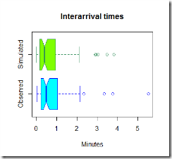
Now that we have uploaded the data, it is time to simulate some observations and compare them to the real one. Below in green is the simulated data.

The code used to simulate the data is here below

Now, the graphs above are pretty, but they are not much use, we need to compare the two sets of graphs to get an idea if our model is fine for this simple task.

 

It looks like our model tends to overestimate the number of arrivals in the 0-0.5 minutes section, however this is just one simulation and the average arrival time is close to what we expected using this model. It seems reasonable to use this distribution to estimate the inter-arrival times and the number of people arrived in the shop.

The R-code

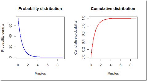
Finally, let's have a look at the ideal exponential distribution given the estimated parameters. Note that some adjustments are necessary because our model is set so that the simulated times are hours, but for practical purposes it is better to work with minutes. Furthermore, by using the exponential distribution formulas we can calculate some probabilities.

By running the code we find out that the probability of the waiting time being less than 3 minutes is 0.975 meaning that it is very likely that one customer group will show up in less than three minutes.

Conclusions.

This model is very basic and simple, both to fit and to run, therefore is very fast to implement. It can be useful to optimize the number of personnel in the store and their function, according to the expected inflow of customers and the average time needed to help the current customers. The hypothesis seem reasonable, given the time of the day considered and provided that the shop does not make some promotion or discount or any other event that could suggest a different behaviour of customers (for instance when there is a discount, it is likely that customers might tell each other to visit the store). For different times of the day, different parameters could be estimated by gathering more data and fitting different exponential distributions.

Complex functions and flow around a cylinder

Last semester I attended a course in complex analysis and I was introduced to the basics tool used in this field. I was fascinated by almost anything that I was taught and although some topics were a little bit difficult to grasp, I am sure it was worth it all the way. Complex Analysis is great for many applications, it is a very powerful tool that enables you to solve problems in the real domain that you would have not otherwise been able to solve.

Among the many applications of complex functions, potential flow is one that took my attention, mainly because it is easygoing for a novice in this field (as I am) but also because of the nice graphs one can plot using it and their physical interpretation.

While looking up for some materials I stumbled upon this paper.

It is quite a nice piece of paper, since it gives a little bit of introduction to complex functions and how they can be used to model flow.

An ideal flow is a flow that is both incompressible and irrotational, that’s to say, if F represents the fluid velocity at each point (x,y), then the following conditions must hold in order for the flow to be ideal:

The conditions above require that the flow has no vorticity (curl) and that the volume of the fluid does not change as it flows (divergence equal to zero).

Theorem 4.5 in the paper connects the velocity vector field and complex (analytic) functions. By then integrating the velocity one can find out the streamlines of the fluid flow.

If the velocity F(z) admits a complex anti-derivative,

and

Therefore the gradient of phi is equal to F and the real part phi(x,y) defines a velocity potential for the fluid flow. The harmonic conjugate psi(x,y) to the velocity potential, in fluid mechanics, is known as the stream function.

Example (4.8). Consider the complex potential function

By making some calculations we can find out

with streamlines

asymptotically horizontal at large distances.

By using Matlab, I implemented this example and plotted some plots about our Gamma function:

 

Now we plot the velocity (gradient of the real part of Gamma) and the the streamlines (psi).

Last but not least, the contour plot of the absolute value of Gama and of its real and imaginary part.

As you can see, the stream function shows that this model can be a first raw step in the way of modelling flow around a steady cylinder. This model however is far from being perfect: among other assumptions it assumes no friction and laminar flow. Laminar flow  can be assumed when the velocity of the fluid is very low and in many practical application it is not often the case. Anyway, this simple model surely can draw some attention to complex analysis and its tools.

2D heat and wave equations on 3D graphs

While writing the scripts for the past articles I thought it might be fun to implement the 2D version of the heat and wave equations and then plot the results on a 3D graph.
As for the wave equation, Wolfram has a great page which describes the problem and explains the solution carefully describing each parameter. Here is a little animation I made using the solution they described

The code for this example is available to be downloaded here.
As far as the heat equation is concerned, I opted for a classical example where you have a hot spot in the middle of a square membrane and given an initial temperature, the heat will flow away as expected. Note that in the heat equation animation the colorbar does not change as time goes on. This can be edited by moving the colorbar into the animation function.

download the code for the heat equation.

On my youtube channel you can find many other animations of the wave equation.